class: center, middle, inverse, title-slide .title[ # Quantifying barley morphology ] .subtitle[ ## using Euler characteristic curves ] .author[ ### <strong>Erik Amézquita</strong>, Michelle Quigley, Tim Ophelders <br> Elizabeth Munch, Dan Chitwood <br> Dan Koenig, Jacob Landis <br> - ] .institute[ ### Computational Mathematics, Science and Engineering <br> Michigan State University <br> - ] .date[ ### July 31st 2020 ] --- class: inverse # Plant morphology <div class="row"> <div class="column" style="max-width:50%"> <iframe width="375" height="210" src="https://www.youtube-nocookie.com/embed/oM9kAq0PBvw?controls=0" frameborder="0" allow="accelerometer; autoplay; encrypted-media; gyroscope; picture-in-picture" allowfullscreen></iframe> <iframe width="375" height="210" src="https://www.youtube-nocookie.com/embed/V39K58evWlU?controls=0" frameborder="0" allow="accelerometer; autoplay; encrypted-media; gyroscope; picture-in-picture" allowfullscreen></iframe> </div> <div class="column" style="max-width:50%"> <iframe width="375" height="210" src="https://www.youtube-nocookie.com/embed/4GBgPIEDoa0?controls=0" frameborder="0" allow="accelerometer; autoplay; encrypted-media; gyroscope; picture-in-picture" allowfullscreen></iframe> <iframe width="375" height="210" src="https://www.youtube-nocookie.com/embed/qkOjHHuoUhA?controls=0" frameborder="0" allow="accelerometer; autoplay; encrypted-media; gyroscope; picture-in-picture" allowfullscreen></iframe> </div> </div> --- # Topological Data Analysis <div class="row"> <div class="column" style="max-width:25%; font-size: 15px;"> <img style="padding: 25px 0 35px 0;" src="../figs/S019_L0_1.gif"> <p style="font-size: 25px; text-align: center; color: DarkRed;"> Raw Data </p> <ul> <li> X-ray CT </li> <li> Point clouds </li> <li> Time series </li> <ul> </div> <div class="column" style="max-width:40%; padding: 0 25px 0 25px; font-size: 15px;"> <img src="../figs/ecc_X.gif"> <p style="font-size: 23px; text-align: center; color: DarkRed;"> Topological Summary </p> <ul> <li> Euler Characteristic </li> <li> Persistence diagrams </li> <li> Mapper/Reeb graphs </li> <ul> </div> <div class="column" style="max-width:35%; font-size: 15px;"> <img src="../figs/svm_mds_canberra_algerian_everest.png"> <img src="../figs/svm_mds_canberra_multan_white-smyrna.png"> <p style="font-size: 25px; text-align: center; color: DarkRed;"> Analysis </p> <ul> <li> Statistics </li> <li> Machine learning </li> <li> Classification/prediction </li> <ul> </div> </div> --- class: center, middle, inverse # 1. Plant Biology: Barley --- # Barley: since the dawn of agriculture - It is the 4th most cultivated grain in the world, behind rice, wheat, and maize. <div class="row"> <div class="column" style="max-width:35%"> <img src="../figs/barley_grains.png"> <img src="../figs/barley_scotland.jpg"> </div> <div class="column" style="max-width:30%"> <p style="font-size: 15px; text-align: center; color: DimGrey;"> Cuneiform tablets from Mesopotamia depicting barley </p> <img src="../figs/Ancient-Mesopotamia-tablet.jpg"> <img src="../figs/mesopotamian-tablet.jpg"> </div> <div class="column" style="max-width:35%"> <img src="../figs/beerancientegypt.jpg"> <p style="font-size: 15px; text-align: center; color: DimGrey;"> Beer consumption in ancient Egypt </p> </div> </div> --- background-image: url("../figs/barley_domestication.jpg") background-size: 910px background-position: 50% 70% # Diversification of floral morphology --- background-image: url("../figs/composite_hybrid_mixture.jpg") background-size: 400px background-position: 95% 5% # Composite Cross (CC II) <div class="row"> <div class="column" style="max-width:36%"> <img src="../figs/BarleyEars_2_vs_6.jpg"> <p style="font-size: 15px; text-align: center; color: DimGrey;"> 2-row vs 6-row barley </p> </div> <div class="column" style="max-width:64%"> <img src="../figs/barley_world.jpg"> <p style="font-size: 15px; text-align: center; color: DimGrey;"> 28 founder lines </p> </div> </div> - Experiment started in 1929, Aberdeen, Idaho - Maintenance by a number of people at UC Riverside. --- background-image: url("../figs/composite_cross_v_05.svg") background-size: 450px background-position: 95% 50% # Experimental design .pull-left[ - Cross all possilbe 28 parent combinations (F1s) - Self-fertilize the resulting 379 hybrids (F2s) - Plant the progeny of hybrids in different plots and let nature do the rest - Mostly self-fertilization was carried out throughout almost 58 generations - We have records of all plots throughout generations - Measure morphology - DNA sequencing - Which genes are selected for? - How did morphology change? ] --- class: center, middle, inverse # 2. Genetics: Zygosity --- background-image: url("../../biology/figs/focus_DNA.jpg") background-size: 610px background-position: 97% 55% # All we are is DNA .left-column[ The DNA is composed of 4 nucleotides - Adenine (A) - Cytosine (C) - Thymine (T) - Guanine (G) Complementarity - `\(A \leftrightarrow T\)` - `\(C \leftrightarrow G\)` Natural replication mechanism ] --- background-image: url("../../biology/figs/alleles.jpg") background-size: 800px background-position: 50% 60% # Molecular basis of mutations **Alelle:** Variation of a known gene. Difference could be one or more nucleotides. **Mutation:** Change of nucleotides in an allele. Add pineapple to a pizza _(mutation)_ vs calling such monster "Hawaiian" _(allele)_ --- background-image: url("../../biology/figs/mutant_phenotypes.jpg") background-size: 600px background-position: 97% 55% # Rarely, one gene = on trait .left-column[ **trait** = **property** **Phenotype:** Shape of a trait **Cross:** Controlled mating **Wild type:** The phenotype observed in nature **Mutant:** Individual with an altered trait ] --- background-image: url("../../biology/figs/how-are-chromosomes-inherited1.png") background-size: 700px background-position: 65% 95% # Dominance vs recesiveness Chromosomes, and thus **genes**, come in pairs: one copy from each parent. - **Dominant:** One copy of the allele is enough to express a phenotype (A) - **Recessive:** Allele needs two copies to be expressed (a) - **Homozygous:** Organism with a pair of identical alleles (line: A/A or a/a) - **Heterozygous:** Organism with a pair of different alleles (A/a) - **Genotype:** Allelic combination of an organism (A/A, A/a, a/a) Each copy of every chromosome **has the same probability** of being inherited. --- background-image: url("../../biology/figs/mendel_single_gene_ratios.jpg") background-size: 790px background-position: 50% 75% # Selfing an heterozygote --- background-image: url("../../biology/figs/punnett_2_alleles_a.jpg") background-size: 370px background-position: 95% 35% # Same idea for two alleles .pull-left[ - Assuming independence, the phenotypic ratio is `\(9:3:3:1\)` - The genotypic ratio is much more different - *Recall:* Being dominant/recessive does not influence the chance of being inherited - *Mendel's second law:* Gene pairs in **different chromosomes** are grouped independently during the formation of gametes.  ] --- background-image: url("../../biology/figs/tomato_varieties.jpg") background-size: 350px background-position: 90% 85% # Synthetising pure lines .pull-left[ - If we keep selfing heterozygotes, half of their progeny will be homozygous. - Selfing an homozygous produces a genotypic (and phenotypic) invariant. - Not all homozygous are viable. - Multiple genes: - A/A b/b c/c D/D - a/a B/B C/C d/d - Both are homozygous - If left to their own devices, which homozygous combinations are the most successful? ] .pull-right[  ] --- class: inverse, center, middle # 3. Image procesing ## X-ray CT scan 3D images --- background-image: url("../figs/barley_lab_composition.jpg") background-size: 750px background-position: 99% 99% # Raw data: X-ray CT scans .pull-left[ Voxel-based images `\(\sim30\mu m\)` resolution Batch scans - 4 per tray 2Gb+ per raw scan ] --- # _Ad-hoc_ image processing <div class="row"> <div class="column" style="max-width:12%; color: DimGrey; font-size: 15px;"> <img src="../figs/S017_0_original.gif"> <p style="text-align: center"> Original </p> </div> <div class="column" style="max-width:12%; color: DimGrey; font-size: 15px;"> <img src="../figs/S017_1_normal.gif"> <p style="text-align: center"> Normalized </p> </div> <div class="column" style="max-width:12%; color: DimGrey; font-size: 15px;"> <img src="../figs/S017_2_unair.gif"> <p style="text-align: center"> Clean </p> </div> <div class="column" style="max-width:12%; color: DimGrey; font-size: 15px;"> <img src="../figs/S017_3_denoise.gif"> <p style="text-align: center"> Prunned </p> </div> <div class="column" style="max-width:27%; color: DimGrey; font-size: 15px;"> <img src="../figs/S015_alignment.jpg"> <p style="text-align: center"> Labeled </p> </div> <div class="column" style="max-width:21%; color: DimGrey; font-size: 15px;"> <img src="../figs/S019_L0_1.gif"> <p style="text-align: center"> Analysis! </p> </div> </div> -- - 224 raw scans in total - 875 individual barley spikes --- # Analyze seed distribution <div class="row"> <div class="column" style="max-width:63%; padding: 0px 50px;"> <img src="../figs/seeds_batch1.png"> <img src="../figs/seeds_batch2.png"> </div> <div class="column" style="max-width:12%; background-color: DarkRed; padding: 5px; border-radius: 15px 0px 0px 30px;"> <img src="../figs/seed_outlier1.png"> <img src="../figs/seed_outlier2.png"> </div> <div class="column" style="max-width:12%; color: Yellow; text-align: center; font-size: 15px; background-color: DarkRed; padding: 5px;"> <img src="../figs/seed_outlier4.png"> <img src="../figs/seed_outlier6.png"> <p><strong> Outliers </strong></p> </div> <div class="column" style="max-width:12%; background-color: DarkRed; padding: 5px; border-radius: 0px 15px 30px 0px;"> <img src="../figs/S102_1_44_0.png"> <img src="../figs/S129_0_37_0.png"> </div> </div> - `\(\sim38,000\)` clean seeds across 3 generations. - Gen 0 (4K), Gen 18 (27K), Gen 58 (7K) --- background-image: url("../figs/seed_mesh.png") background-size: 250px background-position: 80% 60% # Traditional measures All seeds are oblong: align them based on SVD .pull-left[ - Length - Width - Height - Surface area - Volume - Convex surface area - Convex volume  ] --- # Allometry and Morphological evolution <div class="row"> <div class="column" style="max-width:35%; color: Yellow; font-size: 15px;"> <img src="../figs/linfit_Vol_vs_Length.jpg"> <img src="../figs/linfit_Vol_vs_Width.jpg"> <img src="../figs/linfit_Vol_vs_ConvexArea.jpg"> </div> <div class="column" style="max-width:22%; color: Yellow; font-size: 15px;"> <img src="../figs/boxplot_all_Length.png"> <img src="../figs/boxplot_all_Height.png"> </div> <div class="column" style="max-width:22%; color: Yellow; font-size: 15px;"> <img src="../figs/boxplot_all_Width.png"> <img src="../figs/boxplot_all_Area.png"> </div> <div class="column" style="max-width:22%; color: Yellow; font-size: 15px;"> <img src="../figs/boxplot_all_Vol.png"> <img src="../figs/boxplot_all_ConvexVol.png"> </div> </div> --- background-image: url("../figs/boxplot_founders_Length.png") background-size: 850px background-position: 90% 50% # Differences between founder seeds --- class: inverse, middle, center # 3. Topology ## Euler Characteristic Transform (ECT) --- background-image: url("../../tda/figs/euler_characteristic_2.png") background-size: 450px background-position: 97% 50% # The Euler characteristic .pull-left[ Give a 3D object with `\(V_0\)` vertices, `\(V_1\)` edges, and `\(V_2\)` faces. `$$\chi = V_0 - V_1 + V_2$$` **Betti numbers:** Number of homologically different holes. - `\(\beta_0\)`: Number of component components - `\(\beta_1\)`: Number of cycles - `\(\beta_2\)`: Number of voids `\(\chi = \beta_0 - \beta_1 + \beta_2\)` In general: `\(\chi = \sum_{i=0}^n (-1)^iV_i = \sum_{i=0}^n (-1)^i\beta_i\)` ] --- class: center background-image: url("../../tda/figs/euler_characteristic_variety.jpg") background-size: 900px background-position: 50% 80% # Euler characteristic for different shapes The Euler characteristic is a topological invariant: invariant under smooth transformations. .pull-left[ If the Euler characteristic is **different**, the two spaces must be topologically distinct ] .pull-right[ Two spaces can be topologically distintic but their Euler characteristic **can be the same.** ] --- background-image: url("../figs/ecc_X.gif") background-size: 300px background-position: 90% 60% # Euler characteristic curve (ECC) .pull-left[ - Given a finite simplicial complex `\(M\subset\mathbb{R}^d\)` - A direction `\(\nu\in S^{d-1}\)` - Height filtration `\(M(\nu)_r = \{x\in M: \langle x,\nu\rangle \leq r\}\)` `\(\simeq \{\Delta\in M : \langle x, \nu\rangle\leq r\:\forall \,x\in\Delta\}\)` - Define the ECC as `\(\chi(M,\nu):\mathbb{R}\to\mathbb{Z}\)` `$$\chi(M,\nu)(r) = \chi(M(\nu)_r).$$` ] --- background-image: url("../figs/ect.gif") background-size: 700px background-position: 50% 90% # Euler characteristic transform (ECT) - Define `\(ECT(M): S^{d-1}\to\mathbb{Z}^{\mathbb{R}}\)` with `\(\nu\mapsto\chi(M,\nu)\)` - Concatenate an infinite number of ECCs. --- # Why choose the ECT? -- - Easy to compute: a quick alternating sum. -- [**Theorem _(Turner, Mukherjee, Boyer 2014)_**](https://doi.org/10.1093/imaiai/iau011): The ECT is injective for finite simplicial complexes in 3D. -- [**Theorem _(ibid)_**](https://arxiv.org/abs/1310.1030): The ECT is a sufficient statistic for finite simplicial complexes in 3D. -- *Translation:* - Given all the (infinite) ECCs corresponding to all possible directions, - *Different* simplicial complexes correspond to *different* ECTs. - The ECT effectively summarizes all possible information related to shape. --- class: inverse, center, middle # 5. Machine Learning ## Results on barley seeds --- background-image: url("../figs/pole_directions_102.png") background-size: 350px background-position: 90% 50% # Computing the ECT of seeds .pull-left[ - All seeds are centered and aligned so we can associate directions across images - 74 directions - 32 thresholds per direction - Every seed is associated a `\(74\times32=2368\)`-dimensional vector.  ] --- background-image: url("../../demat/figs/pca_figure.jpg") background-size: 290px background-position: 99% 90% ## Unsupervised: Principal Component Analysis (PCA) - Consider `\(\mathbf x_1,\ldots,\mathbf x_n\in\mathbb R^d\)` (say `\(d=2368\)`) -- - Let `\(1\leq k \leq d\)` fixed. Say `\(k=2\)`. -- - We want to find the _best_ __affine__ `\(k\)`-dimensional approximation `\(U\beta + \mu\)` such that the columns form an `\(U = [u_1, \ldots, u_k]\in\mathbb R^{d\times k}\)` orthonormal basis. -- - Optimization problem: `$$\min_{\beta,\mu, U} \sum_{i=1}^n\|x_i - (\mu + U\beta_i)\|^2$$` such that `\(U^\top U=I\)` and `\(\sum_i\beta_i=0\)`. --- ## Unsupervised: MultiDimensional Scaling (MDS) - Consider a symmetric matrix `\(D = (d_{ij}) \in\mathbb R^{n\times n}\)` corresponding to all pairwise **distances** of a data set `\(\mathbf x_1,\ldots,\mathbf x_n\in\mathbb R^d\)` (say `\(d=2368\)`) -- - Let `\(1\leq k \leq d\)` fixed. Say `\(k=2\)`. - We want to find points `\(\mathbf z_1,\ldots,\mathbf z_n\in\mathbb R^k\)` such that their Euclidean distances preserves the original distances as _best_ as possible. -- - Optimization problem `$$\min_{\mathbf z_i\in\mathbb R^k} \sum_{i,j}(\|\mathbf z_i-\mathbf z_j\|_2 - d_{ij})^2$$` such that `\(\sum_{i}\mathbf z_i = 0\)` -- - MDS can be used for dimension reduction. --- background-image: url("../../demat/figs/separable-svm.svg") background-size: 450px background-position: 50% 99% ## Supervised: Support Vector Machines (SVM) - `\(n\)` labeled points `\(\{\mathbf x_i,y_i\}_{i=1}^n \subset \mathbb R^d\)` with `\(y_i\in\{-1,+1\}\)`. -- - We want the __hyperplane H__ that splits the data the _best_, with `\(\mathbf H = \{\mathbf x\,:\,\langle\mathbf{x,w}\rangle+b=0\}\)`. -- - Optimization problem `$$\begin{align} \min_{(\mathbf w,b)\in\mathbb R^d\times\mathbb R}\;\; &\frac12||\mathbf w||^2, \\ \textrm{tal que }\;\;& y_i(\langle \mathbf x_i,\mathbf w\rangle + b)\geq 1 \textrm{ para todo } i=1,\ldots,n. \end{align}$$` --- background-image: url("../figs/confusion_matrix_traditional_crop.png") background-size: 450px background-position: 97% 95% # SVM with traditional measures .pull-left[ - How different are the founder seeds from each other? - SVM to distinguish 28 classes simultaneously. - Each seeds is associated to an `\(11\)`-dimensional vector. - (Take 80% as training and 20% as test) `\(\times\)` 50 times. - Roughly `\(54\%\)` overall classification accuracy. - Confusion happens with hybrids and geographical relatives. ] .pull-right[  ] --- background-image: url("../figs/confusion_matrix_combined_crop.png") background-size: 450px background-position: 97% 95% # Same idea with topology .pull-left[ - With MDS, reduce the ECT information to just 32 dimensions. - The curse of dimensionality is real. - Repeat SVM procedure with only topological information only. - Actually we get just `\(46\%\)` accuracy this time. - Overall confusion structure remains the same - Confusion happens between 2-row founders ] .pull-right[  ] --- # MDS + SVM .pull-left[ - Focus on two founders at a time - Project each ECT to 2D with a metric MDS. - `\(d(\mathbf x, \mathbf z) = \sum_i\frac{|x_i-y_i|}{|x_i|+|y_i|}\)` - Compute a linear SVM to gauge the separability of the ECT+MDS signals. - Used 100% of the data set as training. ] .pull-right[ 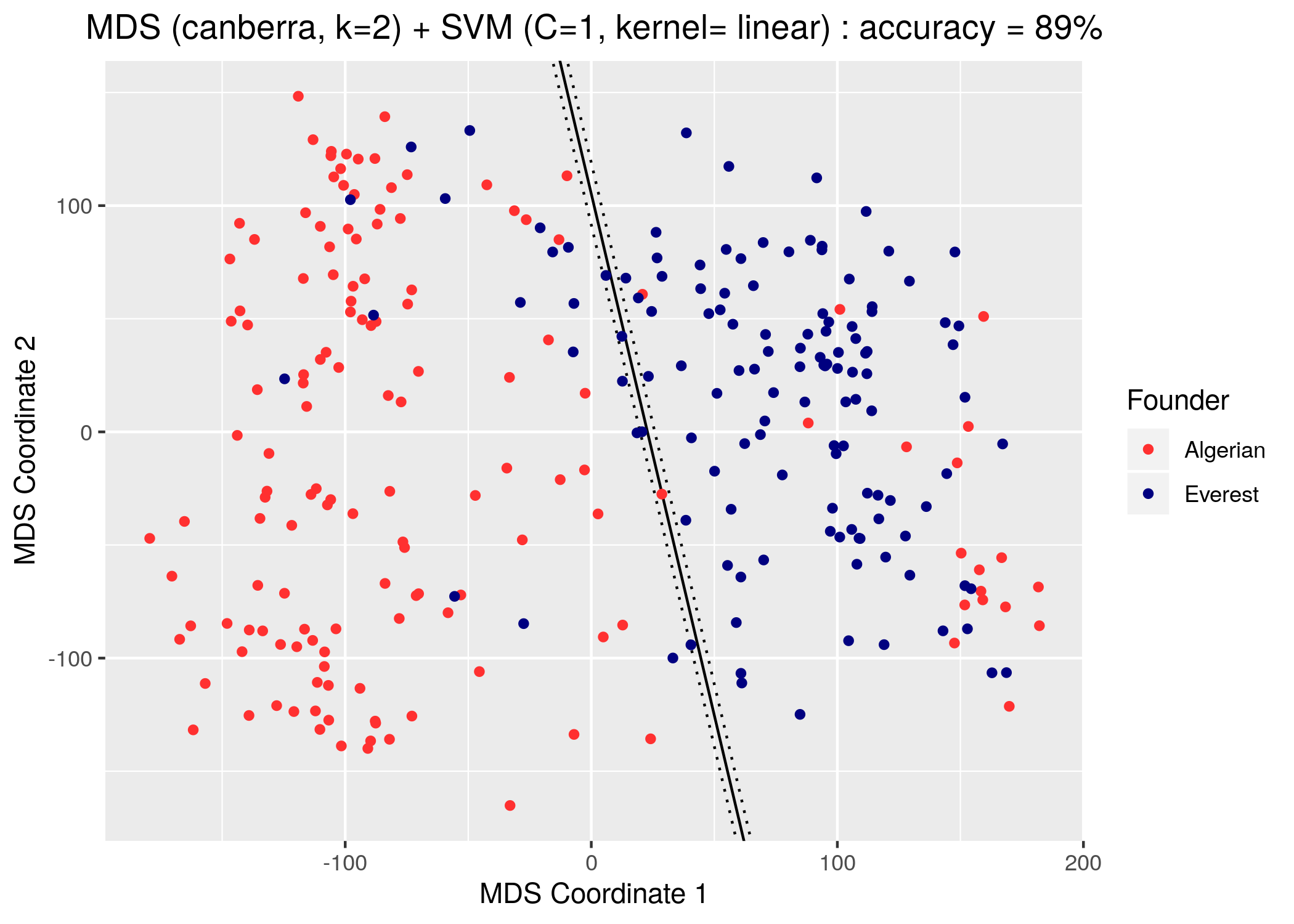 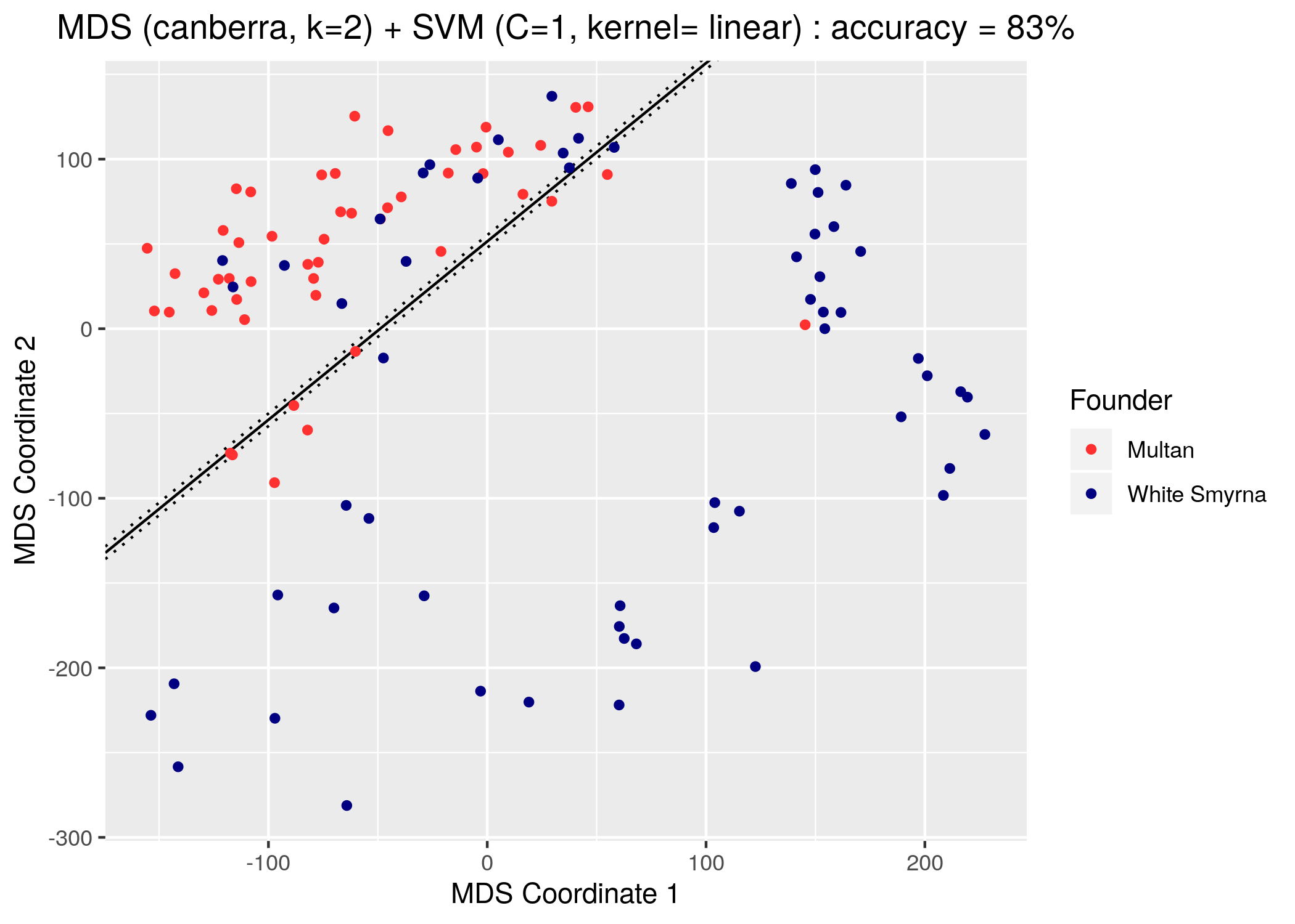 ] --- background-image: url("../figs/heatmap_svm_linear_C1_mds_canberra_k4.png") background-size: 450px background-position: 98% 50% # Accuracy heatmap .pull-left[ Idea: - If two founders are easy to separate, then their morphology must be significantly different. - Thus, such founders ought to be distant in the phylogenetic tree. - The reverse must be true as well. ] --- background-image: url("../figs/hclust_ward.D2_svm_radial_C1_mds_manhattan_k4.png") background-size: 450px background-position: 99% 50% # Hierarchical clustering .pull-left[ - 2-row barley founders tend to cluster - The behavior is mantained as we modify: - Number of projected dimensions with MDS: `\(k=2,4,8\)` - Canberra or Manhattan distance for metric MDS - Radial or linear SVM - Different hierarchical clustering criteria (complete, average, ward, mcquitty) ] --- background-image: url("../figs/founders_rownums2_pca_d74_T32.png") background-size: 450px background-position: 99% 60% # PCA suggests a slight asymmetry. .pull-left[ - It seems that the 6-row barley is slightly more spread along the PC2 axis. - Hypothesis: The lateral seeds in the 6-row barley present a natural asymmetry/handedness.  ] --- class: inverse, center, middle # 6. Bonus ## Wearing a morphometrician hat --- background-image: url("../figs/BarleySeed.svg") background-size: 450px background-position: 99% 60% # Procrustes shape analysis .pull-left[ - Procrustes was mythical fiend who would make sure you fit in his bed. - Define landmarks corresponding to interesting points on every individual. - Rotate, translate, and scale so that overlap difference is minimized - Actually, the collection of landmarks can be thought as representing a "cannonical" shape in a high-dimensional non-Euclidean manifold.  ] --- # Asymmetry between 2-row and 6-row .pull-left[  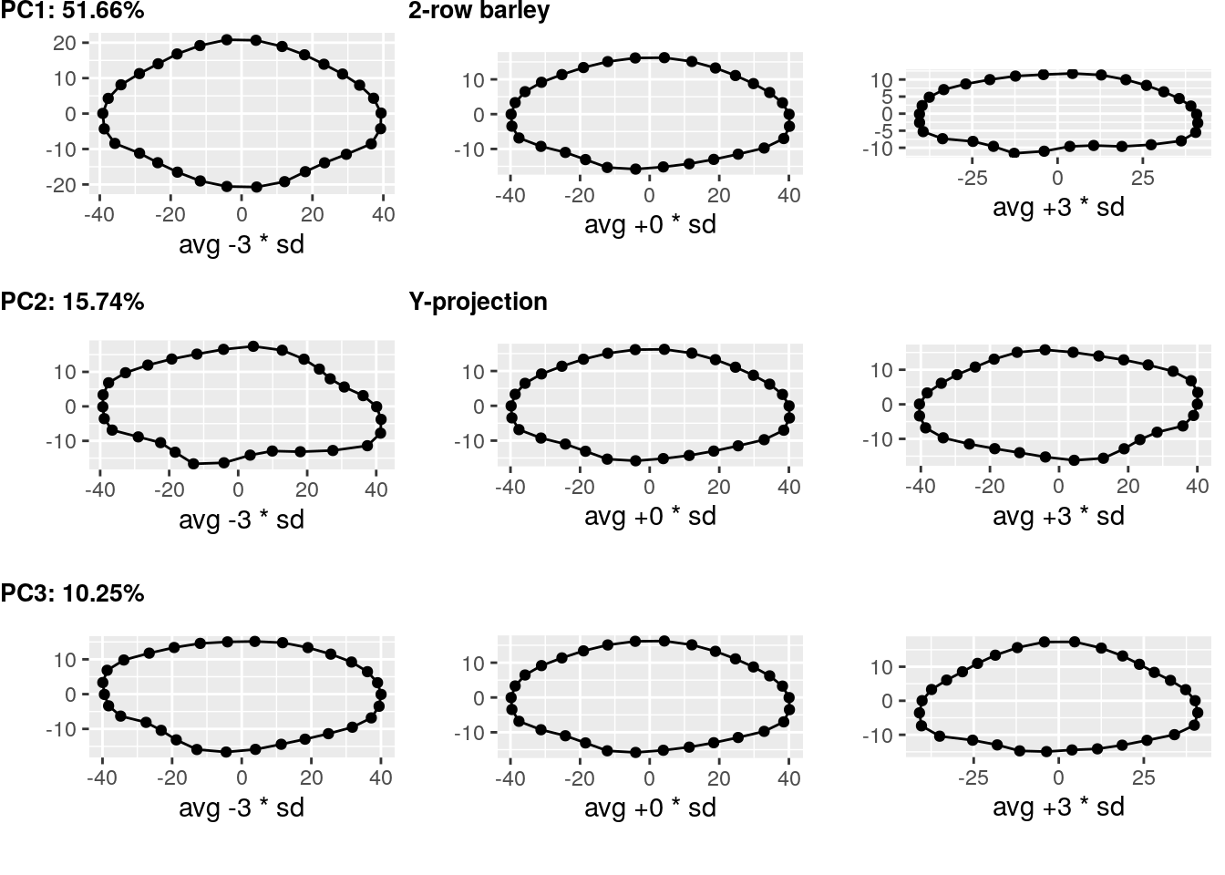 ] .pull-right[ 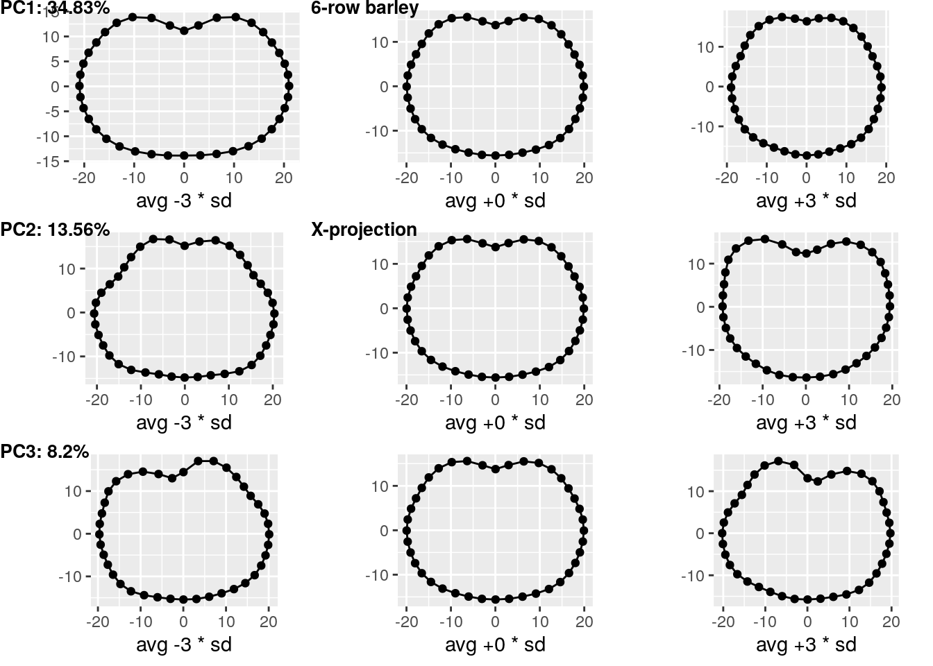 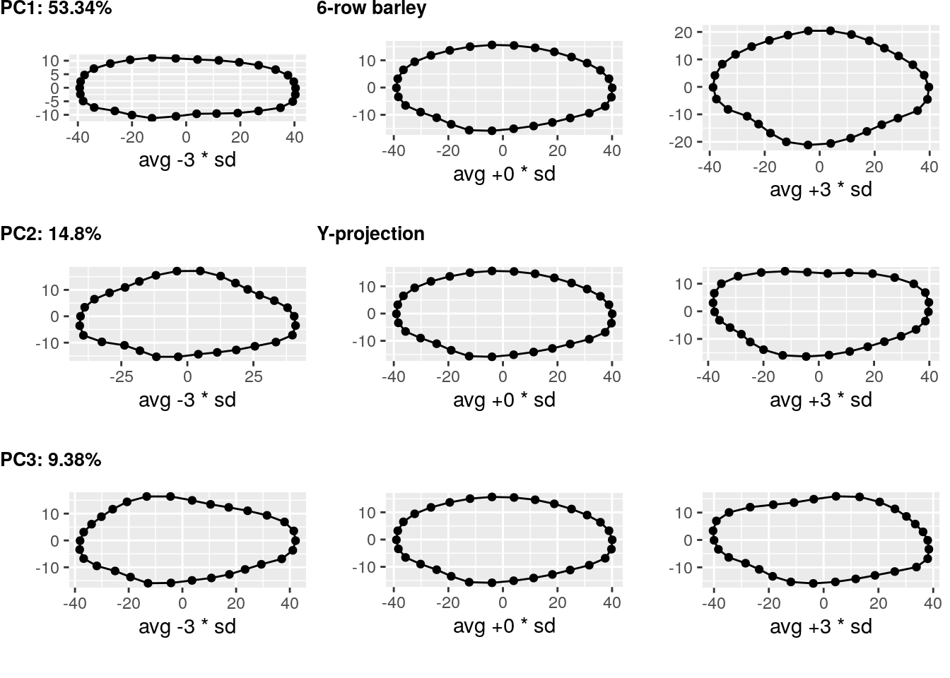 ] --- background-image: url("../figs/gpa_founders_yproj.png") background-size: 450px background-position: 99% 55% # There is something going on with the Y projection .pull-left[ - Consider the PCA of the tangential (Kendall) coordinates of the Y-projection landmarks - The first two PCs explain more than 2/3rds of the total variance - The second PC only accounts for 17% of variance, but it seems to split 2-vs-6 row barley - The other 2 projections didn't show anything similar ] --- # Procrustes analysis only with one row at a time .pull-left[ 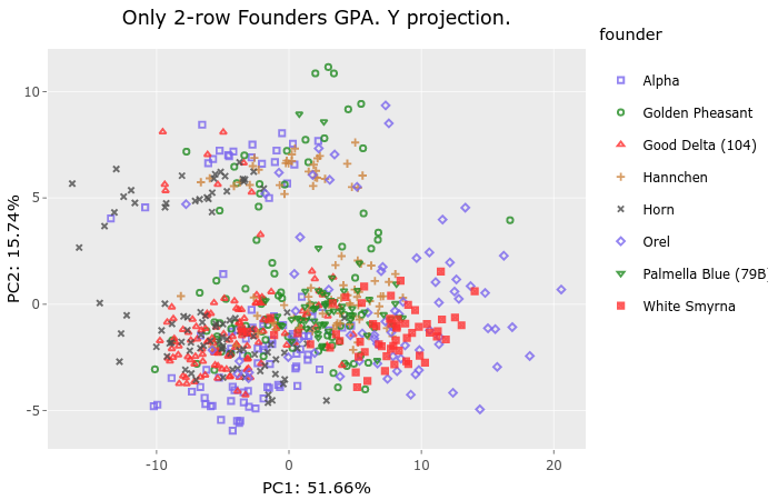 ] .pull-right[ 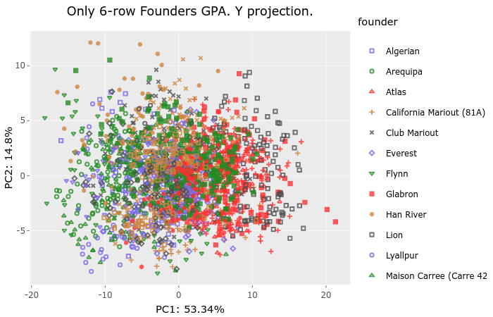 ] - PC1 distinguishes founders. - Each of the 2-row founders is split into two clusters along PC2. - Unclear on how interpret the results. --- class: inverse # Future work - Combine traditional and topological measures to increase classification accuracy -- - Transfer learning: train on founders to predict progeny -- - Do a 3D Procrustes analysis to analyze seed handedness -- - Figure out how to use the barley spike as a whole -- - Find a more concrete link between morphology and genomics -- - Many more plant morphology data sets to be analyzed! <div class="row"> <div class="column" style="max-width:50%"> <iframe width="375" height="210" src="https://www.youtube-nocookie.com/embed/ikhuvGpJbeA?controls=0" frameborder="0" allow="accelerometer; autoplay; encrypted-media; gyroscope; picture-in-picture" allowfullscreen></iframe> </div> <div class="column" style="max-width:50%"> <iframe width="375" height="210" src="https://www.youtube-nocookie.com/embed/a7JCIJRpF8U?controls=0" frameborder="0" allow="accelerometer; autoplay; encrypted-media; gyroscope; picture-in-picture" allowfullscreen></iframe> </div> </div> --- background-image: url("../figs/acknowledgments.jpg") background-size: 1000px background-position: 50% 50%