class: center, middle, inverse, title-slide .title[ # Characterizing spatial patterns and distributions ] .subtitle[ ## with Topological Data Analysis (TDA) ] .author[ ### <strong>Erik Amézquita</strong>, Sutton Tennant, Sandra Thibivillers, Sai Subhash<br>Benjamin Smith, Samik Bhattacharya, Jasper Kläver, Marc Libault<br>—<br>Division of Plant Science & Technology<br>Department of Mathematics<br>University of Missouri<br>— ] .date[ ### 2024-11-21 ] --- # mRNA localization FTW - **Another regulational mechanism**: Spatial segregation and asymmetrical distribution of mRNA. - Observed various spatial patterns across animal and plant species. .pull-left[ 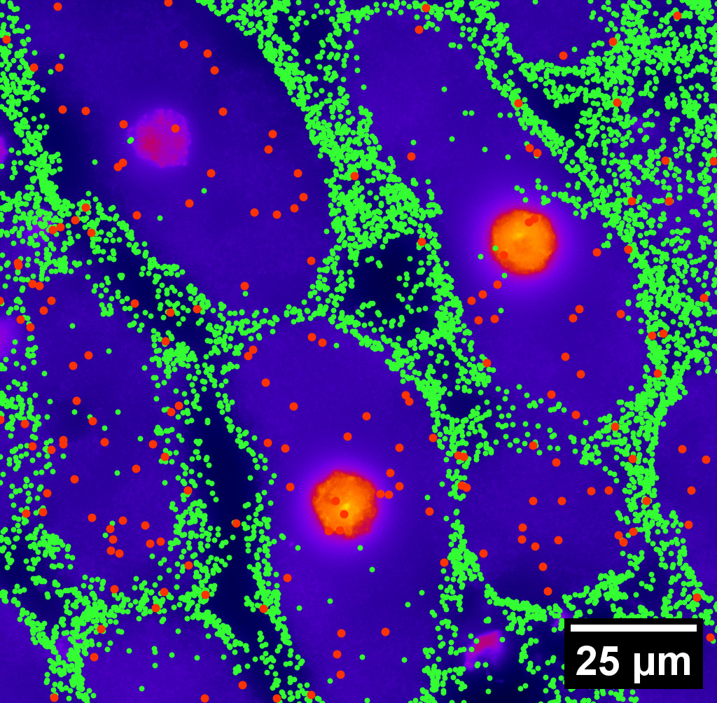 Infected soybean nodule cells. Glyma.05G092200 in green. Glyma.05G216000 in red. ] .pull-right[ - Energetically more efficient to transport mRNA than a whole protein - Efficient protein complex assembly - Prevent proteins from reaching the wrong cellular compartment - Subcellular localization influences proteome architecture and adaptation - mRNA can exert fuctions beyond the protein they encode ] --- # Cellular mechanisms underlying mRNA localization - How does the mRNA end up where it ends up within the cell? .pull-left[ 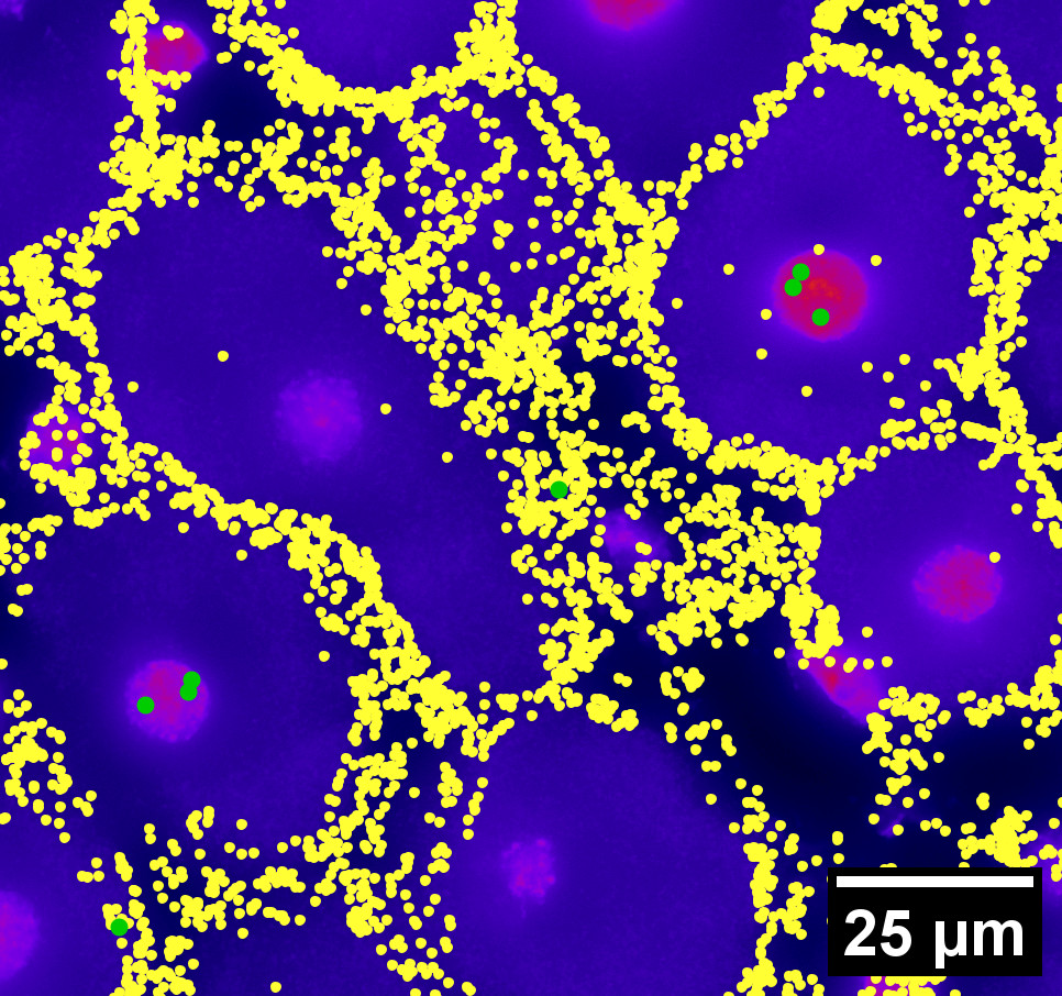 Infected soybean nodule cells. Glyma.05G092200 in yellow. ] .pull-right[ - Motor proteins → Interaction with messenger RNPs (RNA-binding proteins) - General transcript diffusion ⊕ anchoring of RNA at a particular site - All the transcripts are degraded except at a specific region where they are protected - Target transcripts to a specific region ⊕ prevent their access elsewhere ] --- # Molecular mechanisms of mRNA localization control - Mainly RBPs, but ncRNAs, microRNAs, and lncRNCs can partake as well .left-column[ - RNA cis-acting zipcodes - Trans-acting postal workers - Variety of flavors and topologies - Plenty of RNA-RNA interaction to elucidate ] .right-column[ <img src="https://ars.els-cdn.com/content/image/1-s2.0-S0304416517301976-gr3_lrg.jpg" width="400" style="display: block; margin: auto;" /> <p style="font-size: 10px; text-align: right; color: Grey;"> Credits: <a href="https://doi.org/10.1016/j.bbagen.2017.06.011">Chin and Lécuyer (2017)</a></p> ] --- # Different **genes** in different **cells** follow different **spatial patterns** of expression  <p style="font-size: 10px; text-align: right; color: Grey;"> Credits: <a href="https://doi.org/10.1016/j.bbagen.2017.06.011">Chin and Lécuyer (2017)</a></p> - Different cells have different sizes, shapes, and orientations --- # We use Topological Data Analysis (TDA)! 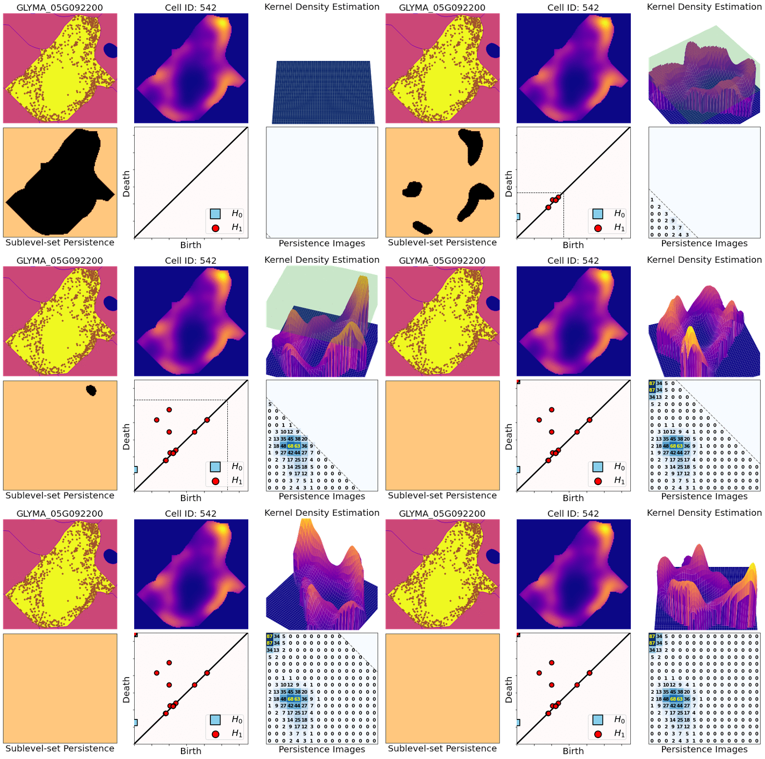 --- class: inverse, middle, center # [1] Molecular Cartography™ # & # Kernel Density Estimators (KDEs) [2] Quantify these heatmaps via Topological Data Analysis (TDA) [3] Link back to biological context --- # Molecular Cartography™  - Soybean nodule 10µm thick cross-sections. - (X,Y,Z) coordinates for 3.7M+ cytosolic transcripts. - 97 genes (including 10 bacterial ones) → 2 genes - 2938 cells → 918 infected ones. - Considered 918 × 2 = 1836 cell-gene pairs --- # Kernel Density Estimations (KDEs) 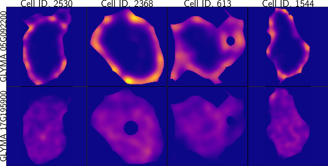 - **Normalize by cell AND gene:** The sum of all transcripts OF ALL genes add to 100% - Each gene adds to a certain percentage - The sum of all genes add to 100% - Compares absolute concentrations --- # "Fixing" 3D data with 2D info  - Consider the Z-axis coordinates of all the bacterial transcripts - Do a 2-sample Kolmogorov-Smirnov test to determine if the putative nuclear and cytosolic transcripts follow the same statistical distribution - If they don't, use the KS statistic as a nuclear-cytosolic breaking point - Proceed **nucleus**-wise --- # "Fixing" 3D data with 2D info <img src="../figs/cell_nucleus_1234.jpg" width="600" style="display: block; margin: auto;" /><img src="../figs/cell_nucleus_2404.jpg" width="600" style="display: block; margin: auto;" /> --- class: inverse, middle, center [1] Molecular Cartography™ & Kernel Density Estimations # [2] Quantify the shape of these heatmaps ## Topological Data Analysis (TDA) and persistent homology [3] Link back to biological context --- # Keep track of blobs `\(H_0\)` and holes `\(H_1\)`  --- # Walking through an example  --- # Walking through an example  --- # Walking through an example  --- # Walking through an example  --- # Walking through an example  --- # Walking through an example  --- # Walking through an example  --- # Walking through an example  --- # Walking through an example  --- # Walking through an example 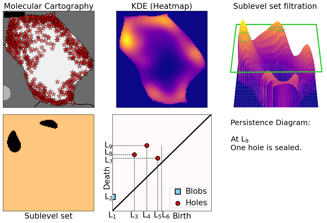 --- # Walking through an example 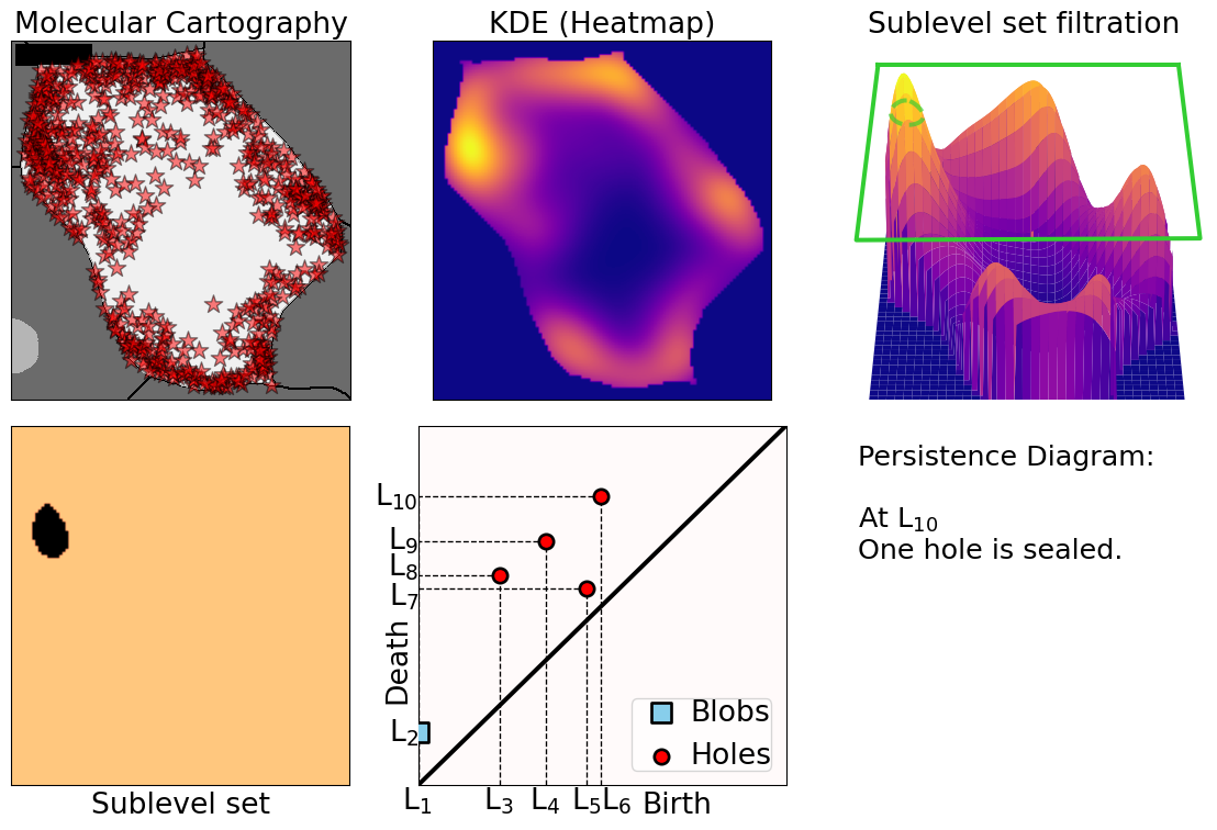 --- # Walking through an example 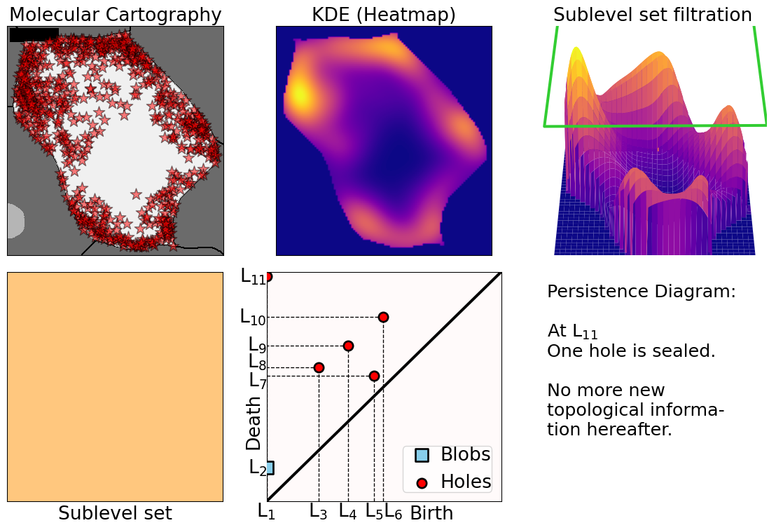 --- # Rotate 45 degrees for ML ammenability 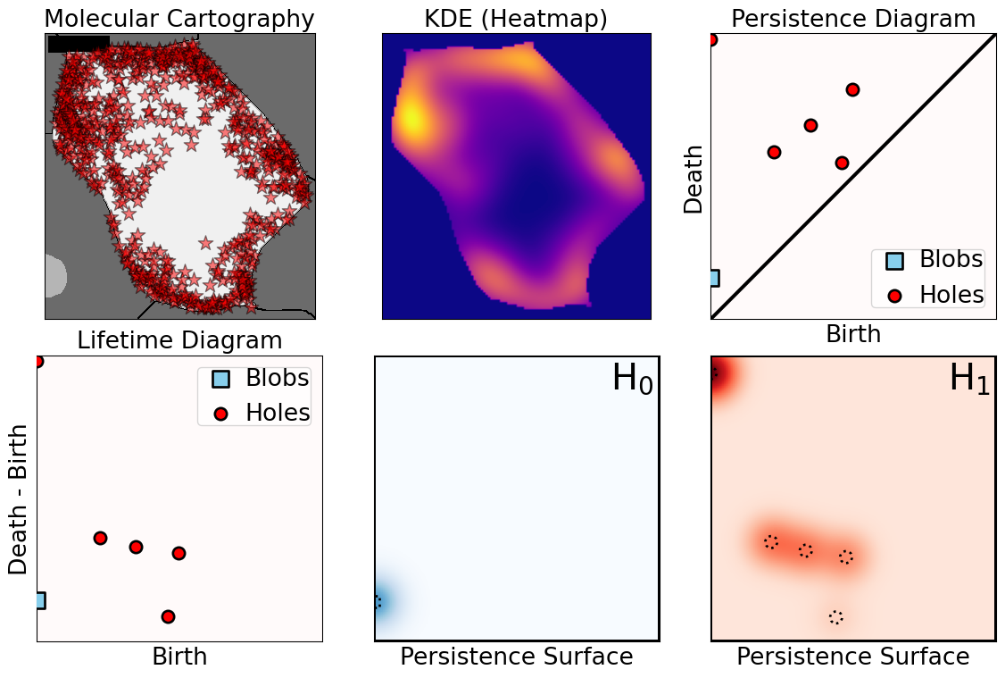 --- # From patterns to numbers 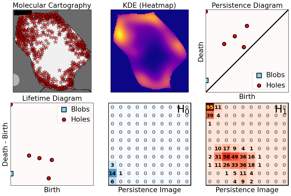 --- # We actually work with 3D data - We keep track of blobs `\(H_0\)`, holes `\(H_1\)`, and voids `\(H_2\)`  <p style="font-size: 10px; text-align: right; color: Grey;"> Credits: <a href="https://commons.wikimedia.org/wiki/File:Earth_Internal_Structure.svg">Wikipedia</a></p> --- # Mathematical justifications - **Definition:** Given two persistence diagrams `\(D_1, D_2\)`, for `\(1\leq p<\infty\)`, we define the *p-Wasserstein* distance between them as `$$W_p(D_1, D_2) := \inf_{\gamma:D_1\to D_2}\left(\sum_{u\in D_1} \left\| u-\gamma(u) \right\|_\infty^p\right)^{1/p},$$` where the infimum is over all possible bijections `\(\gamma: D_1\to D_2\)`. - **Theorem [[Mileyko *et al* (2011)](https://doi.org/10.1088/0266-5611/27/12/124007)]:** For nice filtrations, the persistence diagrams are Wasserstein-stable under small perturbations of the data they summarize. - **Theorem [[Adams *et al.* (2017)](http://jmlr.org/papers/v18/16-337.html)]:** The persistence image `\(I(D)\)` of a persistence diagram `\(D\)` with Gaussian distributions is stable with respect to the 1-Wasserstein distance between diagrams. ### If the overall shape/pattern is perturbed a little bit, then the resulting persistence images are perturbed only a little bit as well --- class: inverse, middle, center [1] Molecular Cartography™ & Kernel Density Estimations [2] Quantify the shape of these heatmaps # [3] Link back to biological context ## Never underestimate the power of PCA --- # Do TDA for all cell-gene combinations <img src="../figs/molecular_cartography_2x4.png" width="500" style="display: block; margin: auto;" /> <img src="../figs/persistence_images_2x4.png" width="600" style="display: block; margin: auto;" /> --- background-image: url("../figs/bw25_scale32_-_PI_1_1_1_H1+2_cell_sample.png") background-size: 620px background-position: 75% 99% # PCA on all topological descriptors <img src="../figs/bw25_both_scale16_-_PI_1_1_1_pca_H1+2_gridded.png" width="350" style="display: block; margin: auto auto auto 0;" /> --- background-image: url("../figs/bw25_scale32_-_PI_1_1_1_H1+2_kde_sample.png") background-size: 620px background-position: 75% 99% # Show me <img src="../figs/bw25_both_scale16_-_PI_1_1_1_pca_H1+2_gridded.png" width="350" style="display: block; margin: auto auto auto 0;" /> --- # Relate back to the biological context 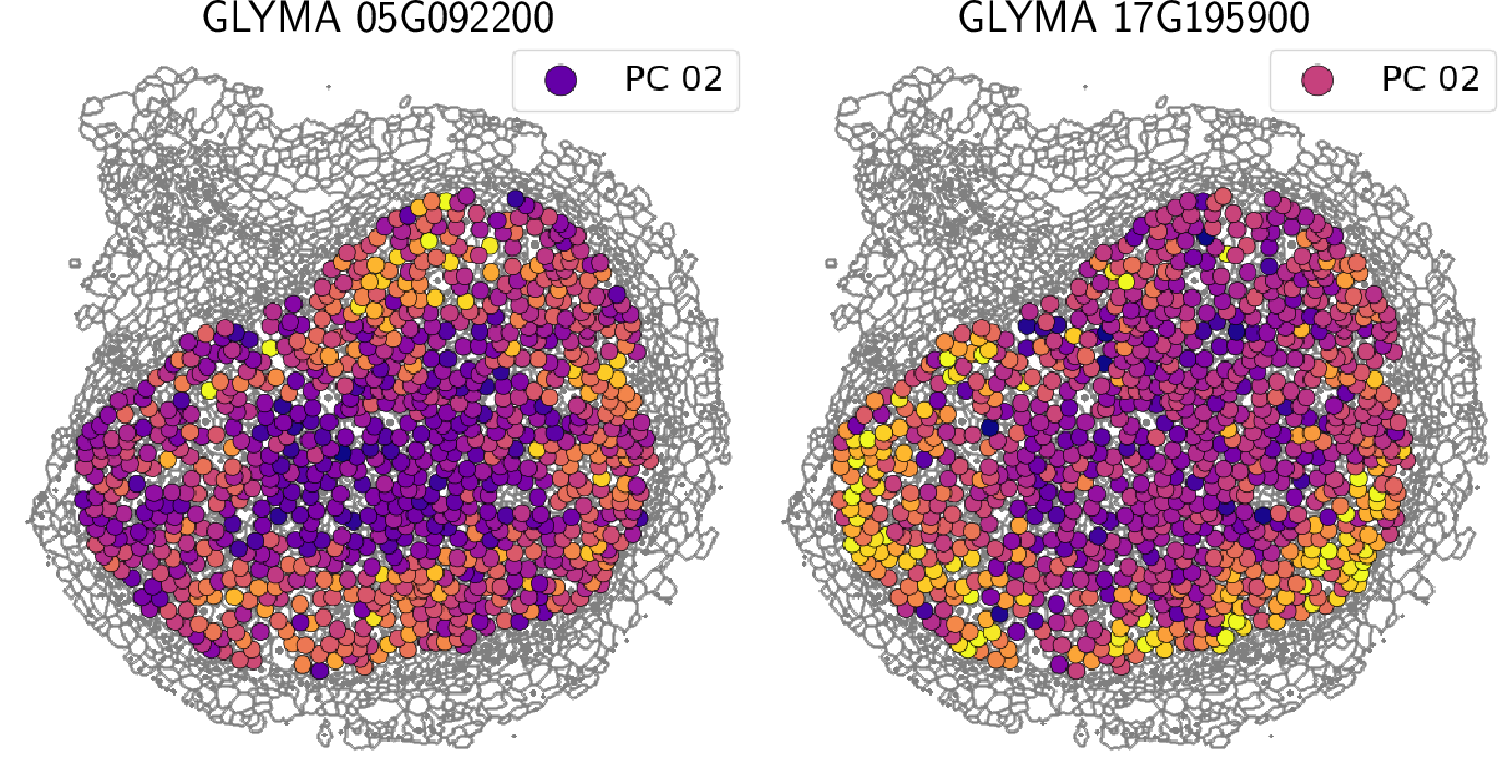 - Senescent cells exhibit a distinct transcriptomic spatial pattern compared to the rest of population. - Loss of mRNA localization may be a lesser known contributor to cell senescence. --- background-image: url("../figs/eccentricity_root_nodule.png") background-size: 300px background-position: 99% 1% # Connecting features to eccentricity --- background-image: url("../figs/eccentricity_root_nodule.png") background-size: 300px background-position: 99% 1% 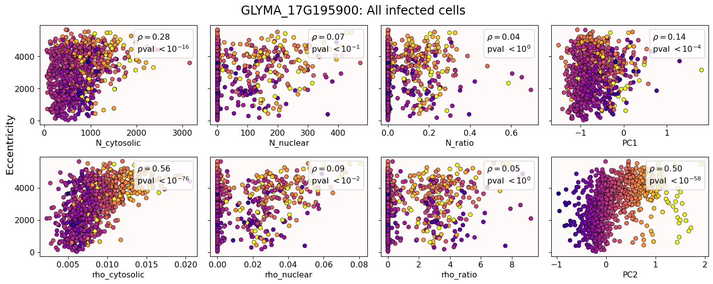 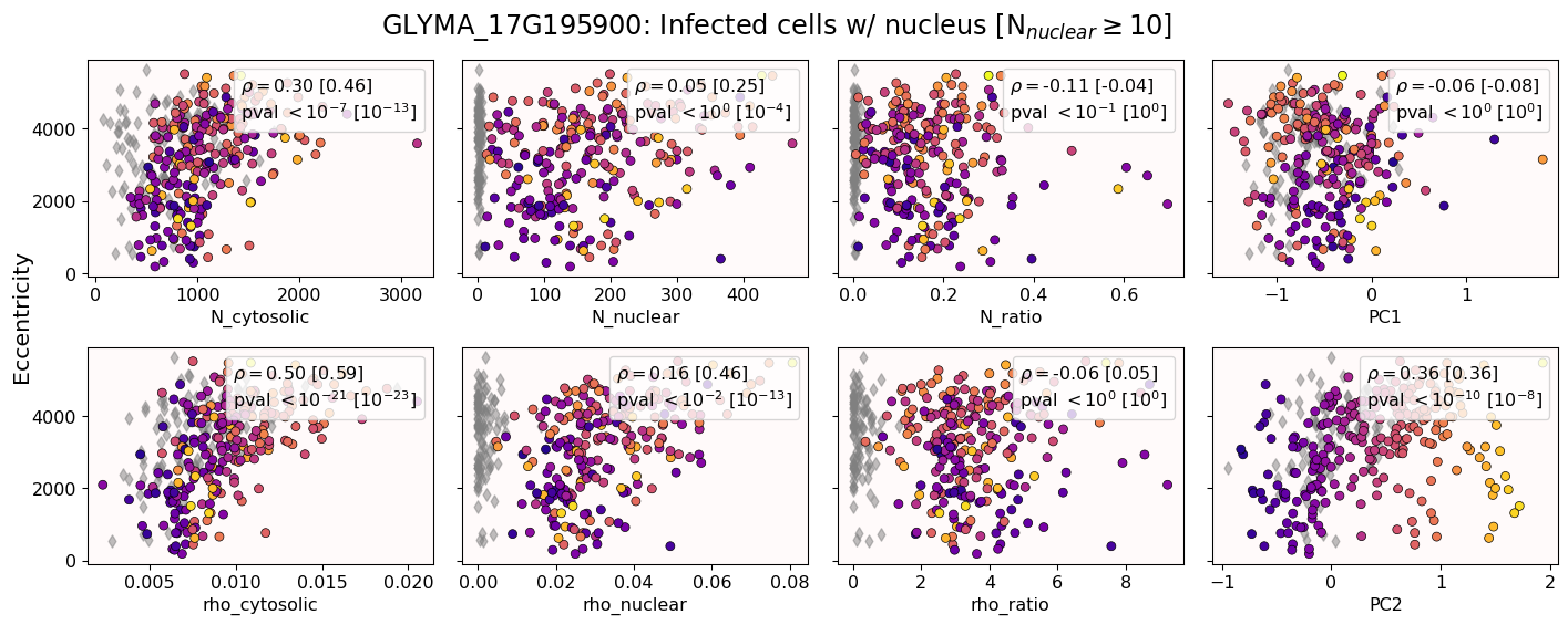 --- background-image: url("../figs/eccentricity_root_nodule.png") background-size: 300px background-position: 99% 1% 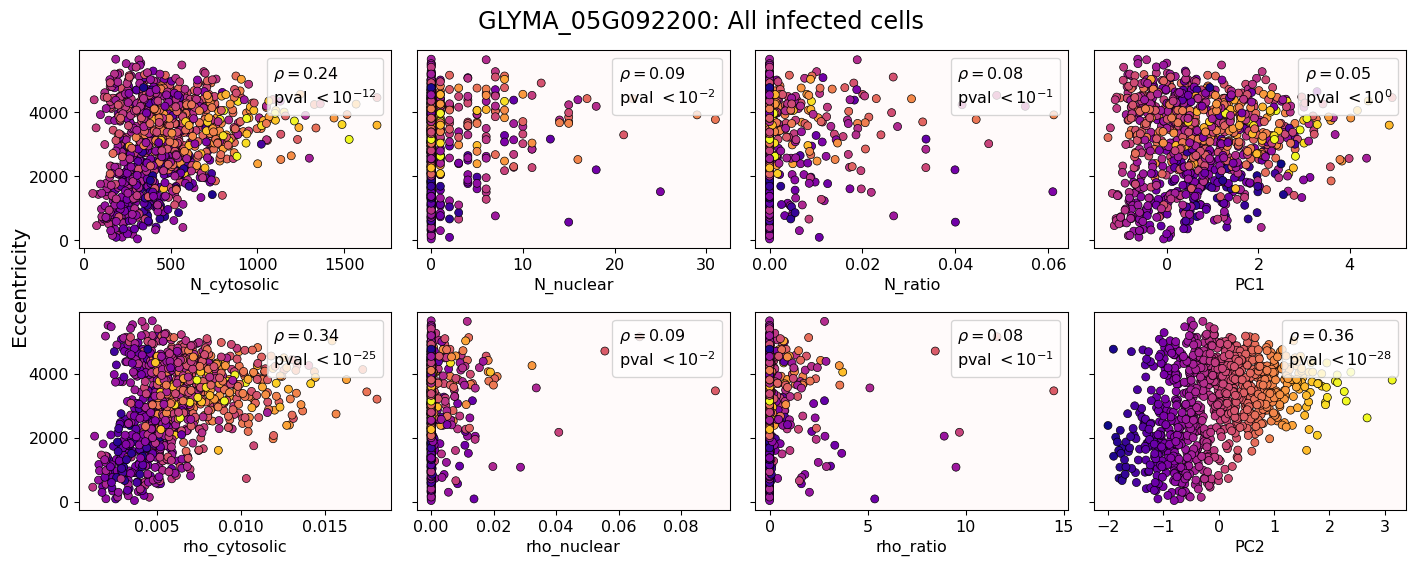 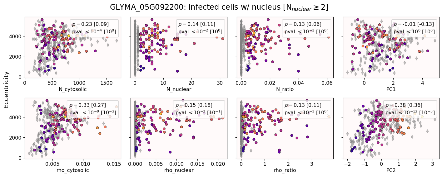 --- # What are the PCs measuring? .pull-left[ 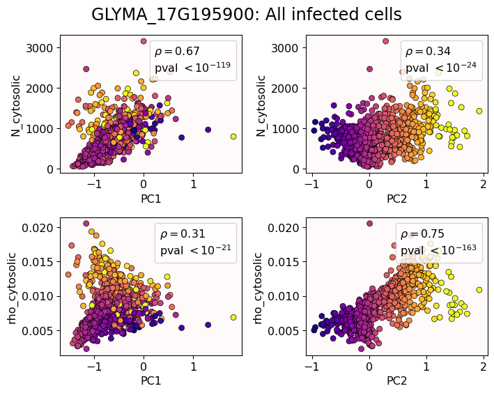 ] .pull-right[ 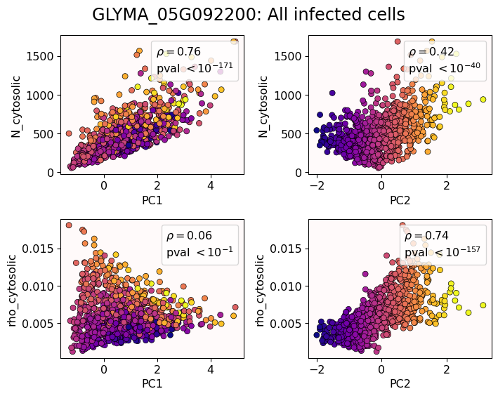 ] -- ## Did I just spent a whole math degree to recompute sample size and transcriptomic density? --- background-image: url("../figs/scale32_-_PI_1_1_1_H1+2_density13_pc02.png") background-size: 600px background-position: 50% 99% # The PCs are capturing other information --- # We define a morphospace of transcriptomic patterns 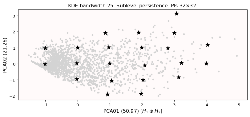 --- class: bottom background-image: url("../figs/scale32_-_PI_1_1_1_H1+2_synthetic_30_clusters.jpg") background-size: 900px background-position: 50% 1% # Working "backward" -- <img src="../figs/scale32_-_PI_1_1_1_H1+2_synthetic_pca_30_clusters.jpg" width="600" style="display: block; margin: auto;" /> --- class: bottom background-image: url("../figs/scale32_-_PI_1_1_1_H1+2_synthetic_varclusters.jpg") background-size: 900px background-position: 50% 1% # Working "backward" -- <img src="../figs/scale32_-_PI_1_1_1_H1+2_synthetic_pca_varclusters.jpg" width="600" style="display: block; margin: auto;" /> --- # Discussion - Topological Data Analysis offers a robust way to encode the *shape of patterns* - Robust to differences in scale, underlying boundaries, or orientation - As long as you have a heatmap, you're good to go: more traditional FISH - Even if you don't, you can make one via KDEs from individual spatial coordinates - Climate patterns? - Canopy patterns? - Cover crop patterns? - Species spatial distribution? 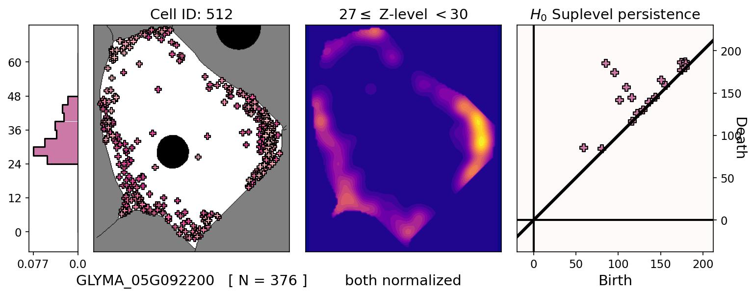 --- # Software used .pull-left[ - All the work has been done in python with mostly standard libries (`numpy`, `scikit-learn`, `matplotlib`, `pandas`, etc.) - KDEs computed efficiently with [`KDEpy`](https://kdepy.readthedocs.io/en/latest/) - Sublevel set filtration of images and persistence diagrams done with [`gudhi`](https://gudhi.inria.fr/)  ] .pull-right[ - Persistence Images computed with [`persim`](https://persim.scikit-tda.org/en/latest/)  ] --- class: inverse # Thank you! <div class="row"> <div class="column" style="max-width:60%; font-size: 15px;"> <img style="padding: 0 0 0 0;" src="https://bondlsc.missouri.edu/wp-content/uploads/2023/11/libault-returns-to-bond-lsc-as-plant-scientist-with-single-cell-focus-1.jpg"> </div> <div class="column" style="max-width:40%; font-size: 24px; line-height:1.25"> <p style="text-align: center;"><strong>Contact and slides:</strong></p> <p style="text-align: center;color:Blue">eah4d@missouri.edu</p> <p style="text-align: center;color:Blue">ejamezquita.github.io</p> </div> </div> <div class="row"> <div class="column" style="max-width:35%; font-size: 20px;"> <p style="font-size: 25px; text-align: center;"> Libault Lab (MU) </p> <ul> <li><strong>Marc Libault</strong></li> <li><strong>Sandra Thibivillers</strong></li> <li>Hengping Xu</li> <li>Sahand Amini</li> <li>Hong Fu</li> <li><strong>Sutton Tennant</strong></li> <li>Md Sabbir Hossain</li> <ul> </div> <div class="column" style="max-width:65%; font-size: 20px;"> <p style="font-size: 25px; text-align: center;"> With help from:</p> <ul> <li>Sai Subash (Nebraska-Lincoln)</li> <li>Benjamin Smith (UC Berkeley)</li> <li>Samik Bhattacharya (Resolve Biosciences)</li> <li>Jasper Kläver (Resolve Biosciences)</li> <ul> </div> </div>