class: center, middle, inverse, title-slide .title[ # Characterizing spatial patterns and distributions ] .subtitle[ ## with Topological Data Analysis (TDA) ] .author[ ### <strong>Erik Amézquita</strong>, Sutton Tennant, Sandra Thibivillers, Sai Subhash<br>Benjamin Smith, Samik Bhattacharya, Jasper Kläver, Marc Libault<br>—<br>Division of Plant Science & Technology<br>Department of Mathematics<br>University of Missouri<br>— ] .date[ ### 2024-12-13 ] --- # Shape has data, and data has shape <div class="row"> <div class="column" style="max-width:19%"> <img src="../../barley/figs/S019_L0_1.gif"></img> <img src="https://botany.one/wp-content/uploads/2018/08/mcy061.jpg"></img> </div> <div class="column" style="max-width:39%"> <iframe width="375" height="210" src="https://www.youtube-nocookie.com/embed/LxNSbrfq3kY?si=Qw9qv3Og1XcPIUyg" title="YouTube video player" frameborder="0" allow="accelerometer; autoplay; clipboard-write; encrypted-media; gyroscope; picture-in-picture; web-share" allowfullscreen></iframe> <img src="../../tda/figs/Mapper_ColorBy_Tissue.png"></img> </div> <div class="column" style="max-width:41%"> <img src="https://i.kinja-img.com/gawker-media/image/upload/s--usj3b0wY--/c_fit,fl_progressive,q_80,w_636/ve69bswtlq7vqih5qrb1.gif"></img> <img src="../../tda/figs/g86.png"></img> </div> </div> --- # We use Topological Data Analysis (TDA)! 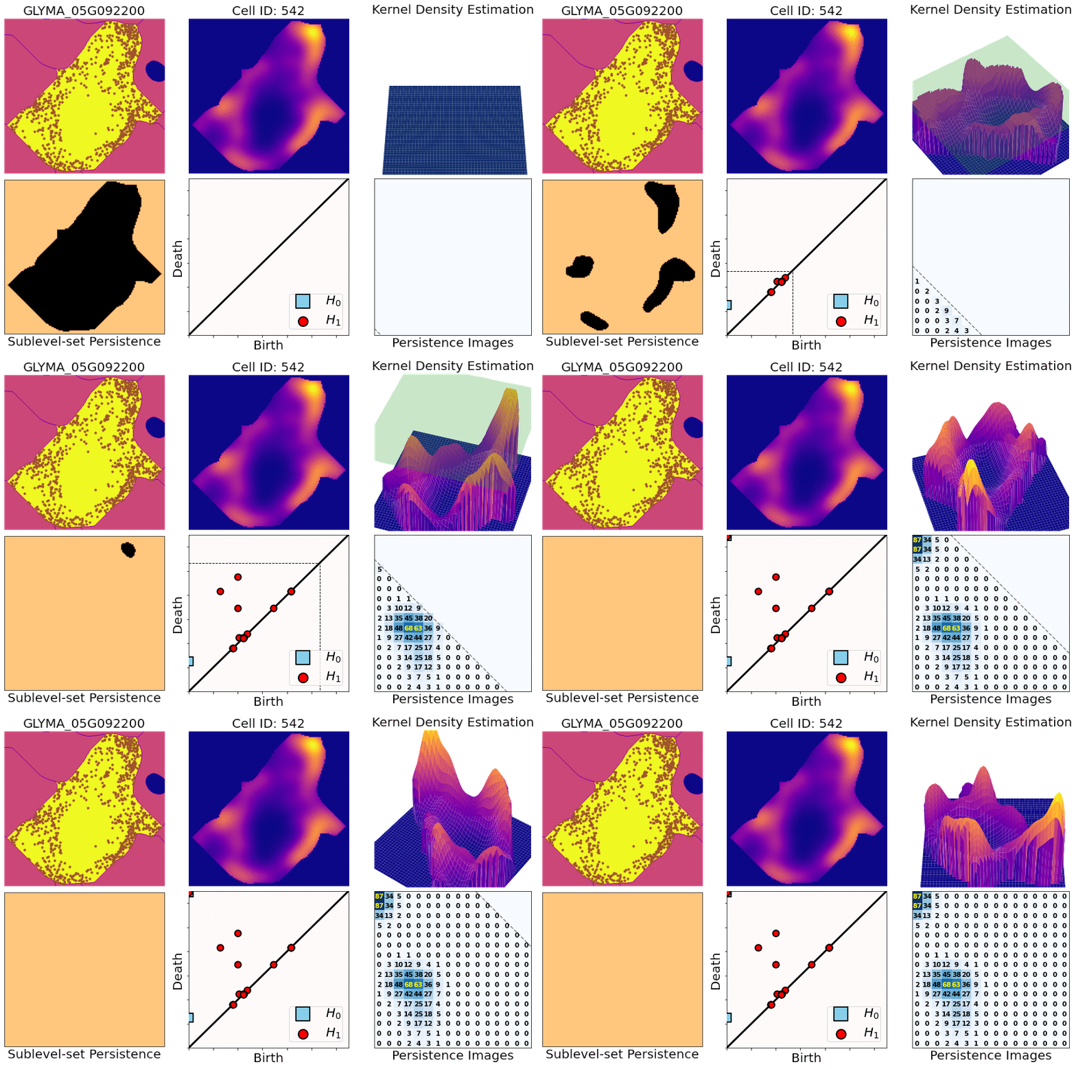 --- background-image: url("../../demat/figs/fam9_3.png") background-size: 100px background-position: 98% 2% # From MX to MI to MO at MU .left-column[  ] .right-column[ - 2013 - 2018 : Licenciatura (Bachelor): Math @ at the Universidad de Guanajuato and CIMAT. Thesis focused on Topological Data Analysis. - 2018 - 2023 : PhD: Computational Mathematics, Science, and Engineering @ Michigan State University. **Came for the math. Stayed for the plants.** - 2023 - Present : PFFIE Postdoc Fellow @ Division of Plant Science & Department of Mathematics at Mizzou ] --- class: inverse, middle, center # Topological Data Analysis ## A primer --- # 1st TDA Ingredient: Complexes - Think the data as a collection of elementary building blocks ( _simplices_ ) Vertices | Edges | Faces | Tetrahedra ---------|-------|-------|------- 0-dim | 1-dim | 2-dim | 3-dim - A collection of cells is a _simplicial complex_ - Count the number of topologically invariant features ( _holes_ ): Connected components | Loops | Voids ---------------------|-------|------- 0-dim | 1-dim | 2-dim - Example with 3 connected components, 1 loop, 1 voids <img src="../../tda/figs/complex-good.svg" width="350" style="display: block; margin: auto;" /> --- # 2nd TDA Ingredient: Filters - Each cell is assigned a real value which defines how the complex is constructed. - Observe how the number of topological features change as the complex grows. .pull-left[ <img src="../../barley/figs/eigcurv_filter.gif" width="250px" style="display: block; margin: auto;" /><img src="../../barley/figs/gaussian_density_filter.gif" width="250px" style="display: block; margin: auto;" /> ] .pull-right[ <img src="../../barley/figs/eccentricity_filter.gif" width="250px" style="display: block; margin: auto;" /><img src="../../barley/figs/vrips_ver2.gif" width="250px" style="display: block; margin: auto;" /> ] --- # Ye olde simplicial homology *with* time - A *filtration* of simplicial complex `\(\mathbf K\)` is a collection of nested subcomplexes `\(\mathbf K_0\subset\mathbf K_0\subset\ldots\subset\mathbf K_m=\mathbf K\)`. <img src="https://www.frontiersin.org/files/Articles/637684/fphys-12-637684-HTML/image_m/fphys-12-637684-g003.jpg" width="400" style="display: block; margin: auto;" /> - We have canonical inclusions `\(\iota_{i,j}:\mathbf K_i\to\mathbf K_j\)`. - We see that `\(\iota_{i,k} = \iota_{j,k}\circ\iota_{i,j}\)` for any `\(0\leq i\leq j\leq k\leq m\)`. - (Abusing notation) These correspond to inclusions `\(\iota_{i,j}:H_q(\mathbf K_i)\to H_q(\mathbf K_j)\)` for `\(q=0,1,2,\ldots\)`. - The `\((i,j)\)`-th persistent `\(q\)`-th homology group is `\(H_{i,j;q}(\mathbf K) = \text{Im}\,(\iota_{i,j})\)`. - It's dimension is the `\((i,j)\)`-th persistent `\(q\)`-th Betti number, `\(\beta_{i,j;q}(\mathbf K)\)`. - A class `\(\alpha\in H_q(\mathbf K_i)\)` *is born* at time `\(i\)` if `\(\alpha\notin H_{i-1,i;q}(\mathbf K)\)`. - This class `\(\alpha\in H_q(\mathbf K_j)\)` *dies* at time `\(j+1\)` if `\(\iota_{j,j+1}(\alpha)\in H_{i,j;q}(\mathbf K)\)`. --- class: inverse, middle, center # An example later will make this much clearer --- # TDA + Biology in the literature <div class="row"> <div class="column" style="max-width:25%"> <img style="padding: 0 0 0 0;" src="https://ars.els-cdn.com/content/image/1-s2.0-S1361841518302688-gr1.jpg"> <img style="padding: 0 0 0 0;" src="https://ars.els-cdn.com/content/image/1-s2.0-S1361841518302688-gr2.jpg"> <p style="font-size: 10px; text-align: right; color: Grey;"> Credits: <a href="https://doi.org/10.1016/j.media.2019.03.014">Qaiser <em>et al.</em> (2019)</a></p> </div> <div class="column" style="max-width:25%"> <img style="padding: 0 0 0 0;" src="https://www.pnas.org/cms/10.1073/pnas.1313480110/asset/ce30e9df-d595-4520-a68a-74f3c6f151d1/assets/graphic/pnas.1313480110fig01.jpeg"> <img style="padding: 0 0 0 0;" src="https://www.pnas.org/cms/10.1073/pnas.1313480110/asset/b733c3a3-00f2-43d5-b372-9da25f3d33c9/assets/graphic/pnas.1313480110fig02.jpeg"> <p style="font-size: 10px; text-align: right; color: Grey;"> Credits: <a href="https://doi.org/10.1073/pnas.1313480110">Chan <em>et al.</em> (2013)</a></p> </div> <div class="column" style="max-width:22%"> <img style="padding: 0 0 0 0;" src="https://www.degruyter.com/document/doi/10.1515/sagmb-2015-0057/asset/graphic/j_sagmb-2015-0057_fig_001.jpg"> <img style="padding: 0 0 0 0;" src="https://www.degruyter.com/document/doi/10.1515/sagmb-2015-0057/asset/graphic/j_sagmb-2015-0057_fig_012.jpg"> <img style="padding: 0 0 0 0;" src="https://www.degruyter.com/document/doi/10.1515/sagmb-2015-0057/asset/graphic/j_sagmb-2015-0057_fig_010.jpg"> <p style="font-size: 10px; text-align: right; color: Grey;"> Credits: <a href="https://doi.org/10.1515/sagmb-2015-0057">Kovacev-Nikolic <em>et al.</em> (2016)</a></p> </div> <div class="column" style="max-width:28%"> <img style="padding: 0 0 0 0;" src="https://media.springernature.com/original/springer-static/image/chp%3A10.1007%2F978-3-030-20867-7_7/MediaObjects/484957_1_En_7_Fig1_HTML.png"> <p style="font-size: 10px; text-align: right; color: Grey;"> Credits: <a href="https://doi.org/10.1007/978-3-030-20867-7_7">Chitwood <em>et al.</em> (2019)</a></p> </div> </div> <div class="row" style="font-family: 'Yanone Kaffeesatz'; font-size:25px;"> <div class="column" style="width:25%;"> <p style="text-align: center;">Holes</p> <p style="text-align: center;">↓</p> <p style="text-align: center;">Cancerous tissue</p> </div> <div class="column" style="width:25%;"> <p style="text-align: center;">Holes</p> <p style="text-align: center;">↓</p> <p style="text-align: center;">Horizontal Reassortment</p> </div> <div class="column" style="width:25%;"> <p style="text-align: center;">Holes</p> <p style="text-align: center;">↓</p> <p style="text-align: center;">Open/closed conformations</p> </div> <div class="column" style="width:25%;"> <p style="text-align: center;">Components</p> <p style="text-align: center;">↓</p> <p style="text-align: center;">Panicle structure</p> </div> </div> --- class: inverse, middle, center # [1] mRNA localization # Molecular Cartography™ ### & # Kernel Density Estimators (KDEs) [2] Quantify these heatmaps via Topological Data Analysis (TDA) [3] Link back to biological context --- # mRNA localization FTW - **Another regulational mechanism**: Spatial segregation and asymmetrical distribution of mRNA. - Observed various spatial patterns across animal and plant species. .pull-left[ 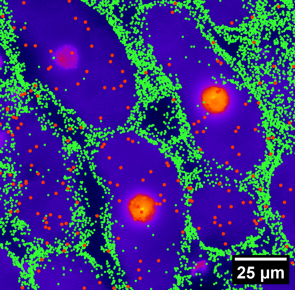 Infected soybean nodule cells. Glyma.05G092200 in green. Glyma.05G216000 in red. ] .pull-right[ - Energetically more efficient to transport mRNA than a whole protein - Efficient protein complex assembly - Prevent proteins from reaching the wrong cellular compartment - Subcellular localization influences proteome architecture and adaptation - mRNA can exert fuctions beyond the protein they encode ] --- # Molecular Cartography™  - Soybean nodule 10µm thick cross-sections. - (X,Y,Z) coordinates for 3.7M+ cytosolic transcripts. - 97 genes (including 10 bacterial ones) → 2 genes - 2938 cells → 918 infected ones. - Considered 918 × 2 = 1836 cell-gene pairs --- # Kernel Density Estimations (KDEs) 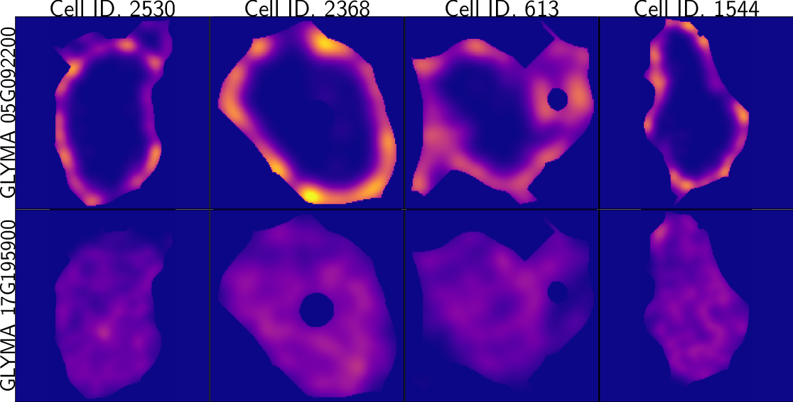 - **Normalize by cell AND gene:** The sum of all transcripts OF ALL genes add to 100% - Each gene adds to a certain percentage - The sum of all genes add to 100% - Compares absolute concentrations --- class: inverse, middle, center [1] Molecular Cartography™ & Kernel Density Estimations # [2] Quantify the shape of these heatmaps ## Topological Data Analysis (TDA) and persistent homology [3] Link back to biological context --- # Keep track of blobs `\(H_0\)` and holes `\(H_1\)`  --- # Walking through an example  --- # Walking through an example  --- # Walking through an example  --- # Walking through an example  --- # Walking through an example  --- # Walking through an example  --- # Walking through an example  --- # Walking through an example  --- # Walking through an example  --- # Walking through an example  --- # Walking through an example 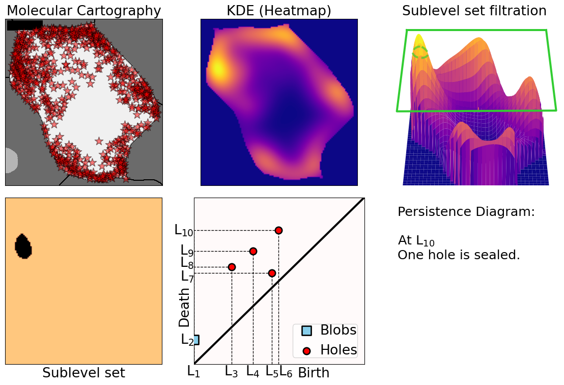 --- # Walking through an example 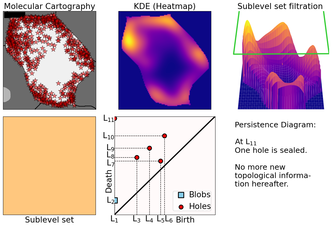 --- # Mathematical motivation: stability - [**Theorem (Cohen-Steiner, Edelsbrunner, Harer, 2007)**](https://doi.org/10.1007/s00454-006-1276-5): Given a nice enough topological space `\(\mathbb{X}\)` and two nice enough filtration functions `\(f,g:\mathbb{X}\to\mathbb{R}\)`, then `$$d_B(\text{dgm}(f), \text{dgm}(g)) \leq \|f-g\|_\infty,$$` - where `\(d_B\)` is the bottleneck distance. - **Translation**: If the original complex wiggles a tiny bit, then the elements of its related persistence diagram will wiggle only a tiny bit as well. ## However - Outside stable distances, it is hard to do anything interesting in the space of persistence diagrams. - E.g.: there are no unique means! - Hard to perform Machine Learning directly with persistence diagrams --- # Rotate 45 degrees for ML ammenability 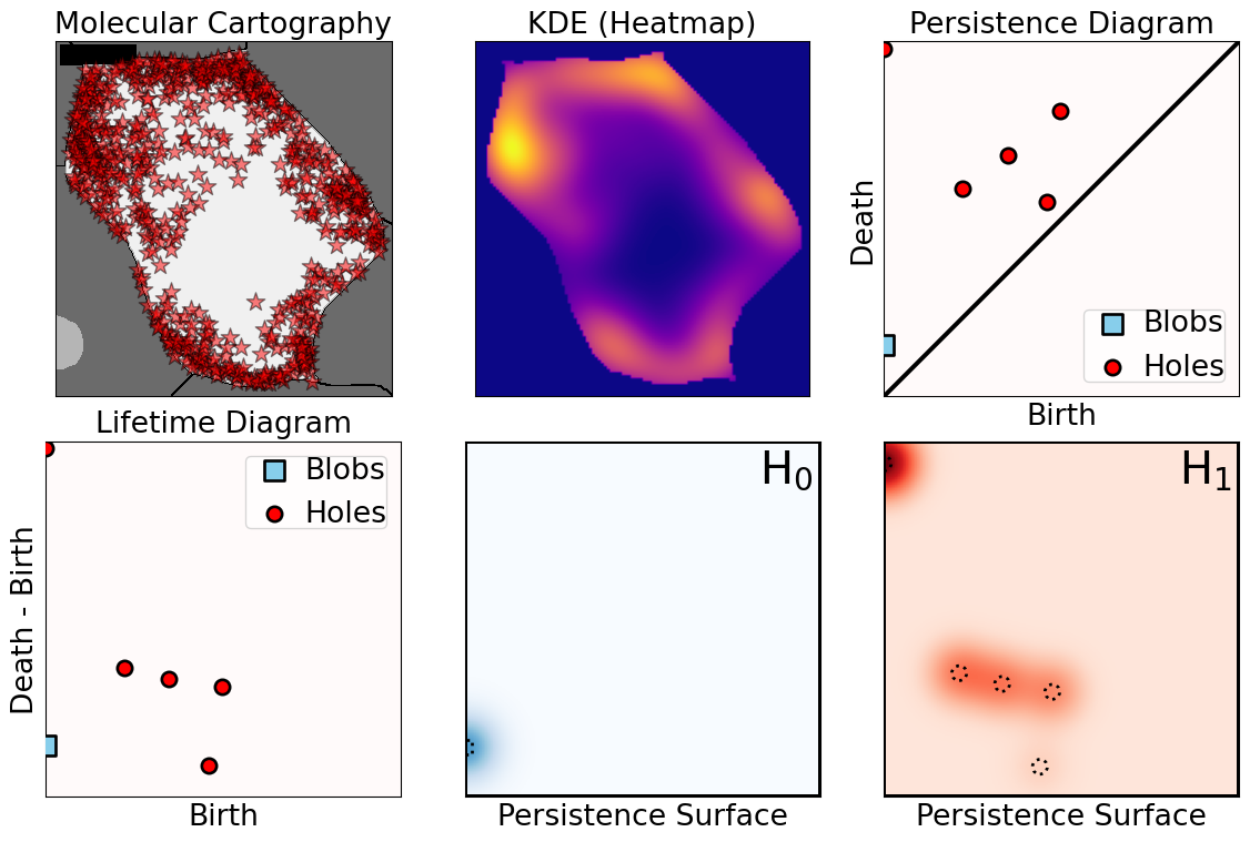 --- # From patterns to numbers 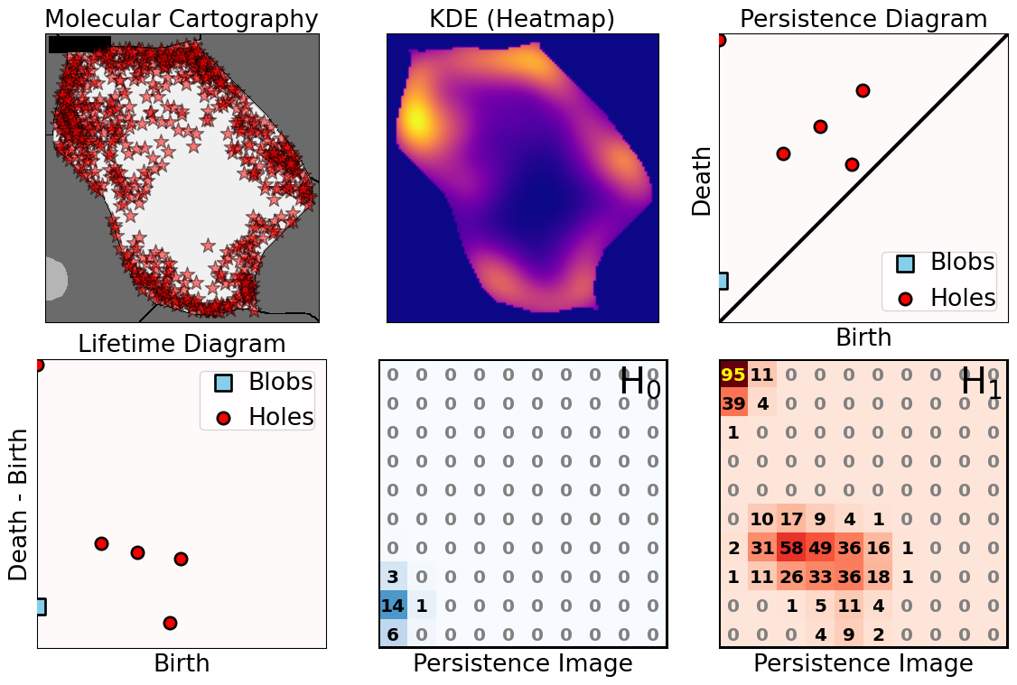 --- # We actually work with 3D data - We keep track of blobs `\(H_0\)`, holes `\(H_1\)`, and voids `\(H_2\)`  <p style="font-size: 10px; text-align: right; color: Grey;"> Credits: <a href="https://commons.wikimedia.org/wiki/File:Earth_Internal_Structure.svg">Wikipedia</a></p> --- # Mathematical justifications - **Definition:** Given two persistence diagrams `\(D_1, D_2\)`, for `\(1\leq p<\infty\)`, we define the *p-Wasserstein* distance between them as `$$W_p(D_1, D_2) := \inf_{\gamma:D_1\to D_2}\left(\sum_{u\in D_1} \left\| u-\gamma(u) \right\|_\infty^p\right)^{1/p},$$` where the infimum is over all possible bijections `\(\gamma: D_1\to D_2\)`. - **Theorem [[Mileyko *et al* (2011)](https://doi.org/10.1088/0266-5611/27/12/124007)]:** For nice filtrations, the persistence diagrams are Wasserstein-stable under small perturbations of the data they summarize. - **Theorem [[Adams *et al.* (2017)](http://jmlr.org/papers/v18/16-337.html)]:** The persistence image `\(I(D)\)` of a persistence diagram `\(D\)` with Gaussian distributions is stable with respect to the 1-Wasserstein distance between diagrams. ### If the overall shape/pattern is perturbed a little bit, then the resulting persistence images are perturbed only a little bit as well --- class: inverse, middle, center [1] Molecular Cartography™ & Kernel Density Estimations [2] Quantify the shape of these heatmaps # [3] Link back to biological context ## Never underestimate the power of PCA --- # Do TDA for all cell-gene combinations <img src="../figs/molecular_cartography_2x4.png" width="500" style="display: block; margin: auto;" /> <img src="../figs/persistence_images_2x4.png" width="600" style="display: block; margin: auto;" /> --- background-image: url("../figs/bw25_scale32_-_PI_1_1_1_H1+2_cell_sample.png") background-size: 620px background-position: 75% 99% # PCA on all topological descriptors <img src="../figs/bw25_both_scale16_-_PI_1_1_1_pca_H1+2_gridded.png" width="350" style="display: block; margin: auto auto auto 0;" /> --- background-image: url("../figs/bw25_scale32_-_PI_1_1_1_H1+2_kde_sample.png") background-size: 620px background-position: 75% 99% # Show me <img src="../figs/bw25_both_scale16_-_PI_1_1_1_pca_H1+2_gridded.png" width="350" style="display: block; margin: auto auto auto 0;" /> --- # Relate back to the biological context  - Senescent cells exhibit a distinct transcriptomic spatial pattern compared to the rest of population. - Loss of mRNA localization may be a lesser known contributor to cell senescence. --- background-image: url("../figs/eccentricity_root_nodule.png") background-size: 600px background-position: 50% 95% # Connecting features to eccentricity --- background-image: url("../figs/eccentricity_root_nodule.png") background-size: 300px background-position: 99% 1%   --- # What are the PCs measuring? .pull-left[  ] .pull-right[ 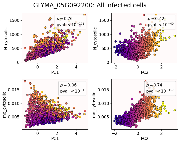 ] -- ## Did I just spent a whole math degree to recompute sample size and transcriptomic density? --- background-image: url("../figs/scale32_-_PI_1_1_1_H1+2_density13_pc02.png") background-size: 600px background-position: 50% 99% # The PCs are capturing other information --- # We define a morphospace of transcriptomic patterns 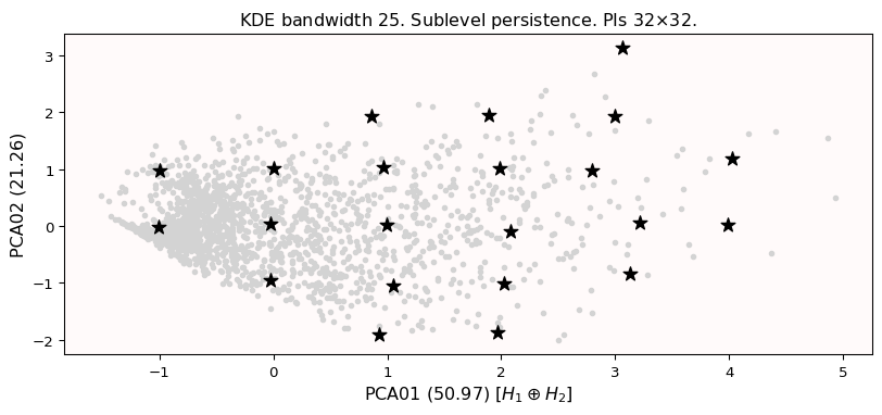 --- class: bottom background-image: url("../figs/scale32_-_PI_1_1_1_H1+2_synthetic_30_clusters.jpg") background-size: 900px background-position: 50% 1% # Working "backward" -- <img src="../figs/scale32_-_PI_1_1_1_H1+2_synthetic_pca_30_clusters.jpg" width="600" style="display: block; margin: auto;" /> --- class: bottom background-image: url("../figs/scale32_-_PI_1_1_1_H1+2_synthetic_varclusters.jpg") background-size: 900px background-position: 50% 1% # Working "backward" -- <img src="../figs/scale32_-_PI_1_1_1_H1+2_synthetic_pca_varclusters.jpg" width="600" style="display: block; margin: auto;" /> --- # Discussion - Topological Data Analysis offers a robust way to encode the *shape of patterns* - Robust to differences in scale, underlying boundaries, or orientation - As long as you have a heatmap, you're good to go: more traditional FISH - Even if you don't, you can make one via KDEs from individual spatial coordinates - Climate patterns? - Canopy patterns? - Cover crop patterns? - Species spatial distribution? 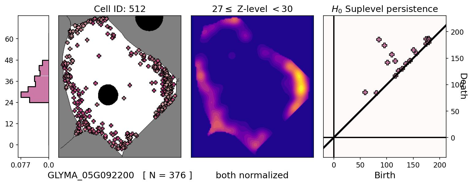 --- # Software used .pull-left[ - All the work has been done in python with mostly standard libries (`numpy`, `scikit-learn`, `matplotlib`, `pandas`, etc.) - KDEs computed efficiently with [`KDEpy`](https://kdepy.readthedocs.io/en/latest/) - Sublevel set filtration of images and persistence diagrams done with [`gudhi`](https://gudhi.inria.fr/)  ] .pull-right[ - Persistence Images computed with [`persim`](https://persim.scikit-tda.org/en/latest/)  ] --- class: inverse # Thank you! <div class="row"> <div class="column" style="max-width:60%; font-size: 15px;"> <img style="padding: 0 0 0 0;" src="https://bondlsc.missouri.edu/wp-content/uploads/2023/11/libault-returns-to-bond-lsc-as-plant-scientist-with-single-cell-focus-1.jpg"> </div> <div class="column" style="max-width:40%; font-size: 24px; line-height:1.25"> <p style="text-align: center;"><strong>Contact and slides:</strong></p> <p style="text-align: center;color:Blue">eah4d@missouri.edu</p> <p style="text-align: center;color:Blue">ejamezquita.github.io</p> </div> </div> <div class="row"> <div class="column" style="max-width:35%; font-size: 20px;"> <p style="font-size: 25px; text-align: center;"> Libault Lab (MU) </p> <ul> <li><strong>Marc Libault</strong></li> <li><strong>Sandra Thibivillers</strong></li> <li>Hengping Xu</li> <li>Sahand Amini</li> <li>Hong Fu</li> <li><strong>Sutton Tennant</strong></li> <li>Md Sabbir Hossain</li> <ul> </div> <div class="column" style="max-width:65%; font-size: 20px;"> <p style="font-size: 25px; text-align: center;"> With help from:</p> <ul> <li>Sai Subash (Nebraska-Lincoln)</li> <li>Benjamin Smith (UC Berkeley)</li> <li>Samik Bhattacharya (Resolve Biosciences)</li> <li>Jasper Kläver (Resolve Biosciences)</li> <ul> </div> </div>