class: center, middle, inverse, title-slide .title[ # Genomics data analysis ] .subtitle[ ## via spectral shape and topology ] .author[ ### <strong>Erik Amézquita</strong>, Farzana Nasrain <br> Katie Storey, Masato Yoshizawa <br> - ] .institute[ ### Plant Sciencs & Mathematics <br> University of Missouri <br> - ] .date[ ### 2023-10-11 <br> - <br> Published in <a href="https://doi.org/10.1371/journal.pone.0284820">PLoS ONE (2023)</a> ] --- ## RNA-seq and the curse of high dimensionality - High-dimensional spaces get really weird really fast - The 10% of a unit cube occupies almost the whole cube at high dimensions - RNA-seq data lies in a 20,000-dimensional space. - Reducing dimension **and clustering** is crucial to understand the data. <img src="../../demat/figs/curse_of_dimensionality.svg" width="600" style="display: block; margin: auto;" /> --- # Mapper **is not** t-SNE, PCA, MDS, etc. - Others only take high-dimensional proximity into account. - They discard overaching shape structure in gene expression profiles. - Mapper **clusters** and **reduces dimension** while preserving the topological shape of the data.  <p style="font-size: 9px; text-align: right; color: Grey;"> Credits: <a href="https://doi.org/10.1142/9789813279827_0032">Wang <em>et al.</em> (2018)</a></p> --- class: inverse, middle, center # Mapper: a toy example ## A Topological Method for the Analysis of High Dimensional Data Sets --- background-image: url("../../tda/figs/mapper_b_00.svg") background-size: 725px background-position: 50% 95% ## Topological summary: exploration and visualization - We start with **lots** of data points `\(X\)` in a **high-dimensional** space - We want just a **handful** of points in a **low-dimensional** space that roughly preserve the original **shape** --- background-image: url("../../tda/figs/mapper_b_01.svg") background-size: 725px background-position: 50% 95% ## Pick a filter function - Assign every data point a **real** value: lens or filter function - We pick *height* in this case --- background-image: url("../../tda/figs/mapper_b_02.svg") background-size: 725px background-position: 50% 95% ## Pick a number of bins and overlap percentages - Split the filter values into a series of **overlapping bins**. - More bins &rarr; better topological resolution but risk of overfitting. --- background-image: url("../../tda/figs/mapper_b_03.svg") background-size: 725px background-position: 50% 95% ## Consider the filter preimages and cluster - Check which data points correspond to the first bin based on their filter values (the preimage) --- background-image: url("../../tda/figs/mapper_b_04.svg") background-size: 725px background-position: 50% 95% ## Consider the filter preimages and cluster - Check which data points correspond to the first bin based on their filter values (the preimage) - **Cluster** the data points in the preimage --- background-image: url("../../tda/figs/mapper_b_05.svg") background-size: 725px background-position: 50% 95% ## Consider the filter preimages and cluster - Check which data points correspond to the first bin based on their filter values (the preimage) - **Cluster** the data points in the preimage - Each cluster will form an individual **node** in our mapper graph --- background-image: url("../../tda/figs/mapper_b_06.svg") background-size: 725px background-position: 50% 95% ## Consider the filter preimages and cluster - Do the same for the next filter bin --- background-image: url("../../tda/figs/mapper_b_07.svg") background-size: 725px background-position: 50% 95% ## Consider the filter preimages and cluster - Do the same for the next filter bin - We have two clusters now --- background-image: url("../../tda/figs/mapper_b_08.svg") background-size: 725px background-position: 50% 95% ## Are there points shared in the overlap? - Draw an edge between mapper nodes if their corresponding clusters **share** data points - *Optional*: The edge thickness (weight) can be proportional to the number of shared points --- background-image: url("../../tda/figs/mapper_b_09.svg") background-size: 725px background-position: 50% 95% ## And so on and so forth - Cluster the data points corresponding to the preimage of a filter bin - Make nodes in the mapper graph --- background-image: url("../../tda/figs/mapper_b_10.svg") background-size: 725px background-position: 50% 95% ## And so on and so forth - Cluster the data points corresponding to the preimage of a filter bin - Make nodes in the mapper graph - Draw edges whenever the clusters share points --- background-image: url("../../tda/figs/mapper_b_11.svg") background-size: 725px background-position: 50% 95% ## Mapper: several moving parts - Filter function - Number of bins - Overlap percentage between bins --- class: inverse, middle, center # Mapper in genomics ## Brief literature survey ### Visualization to inspire new research --- ## Mapper to identify novel groups of breast cancer - Different branches correspond to different molecular profiles and prognosis <p style="font-size: 9px; text-align: right; color: Grey;"> Credits: <a href="https://doi.org/10.1073/pnas.1102826108">Nicolau <em>et al.</em> (2011)</a></p>  --- ## Mapper to differentiate differentiation <p style="font-size: 9px; text-align: right; color: Grey;"> Credits: <a href="https://doi.org/10.1038/nbt.3854">Rivzi <em>et al.</em> (2017)</a></p> 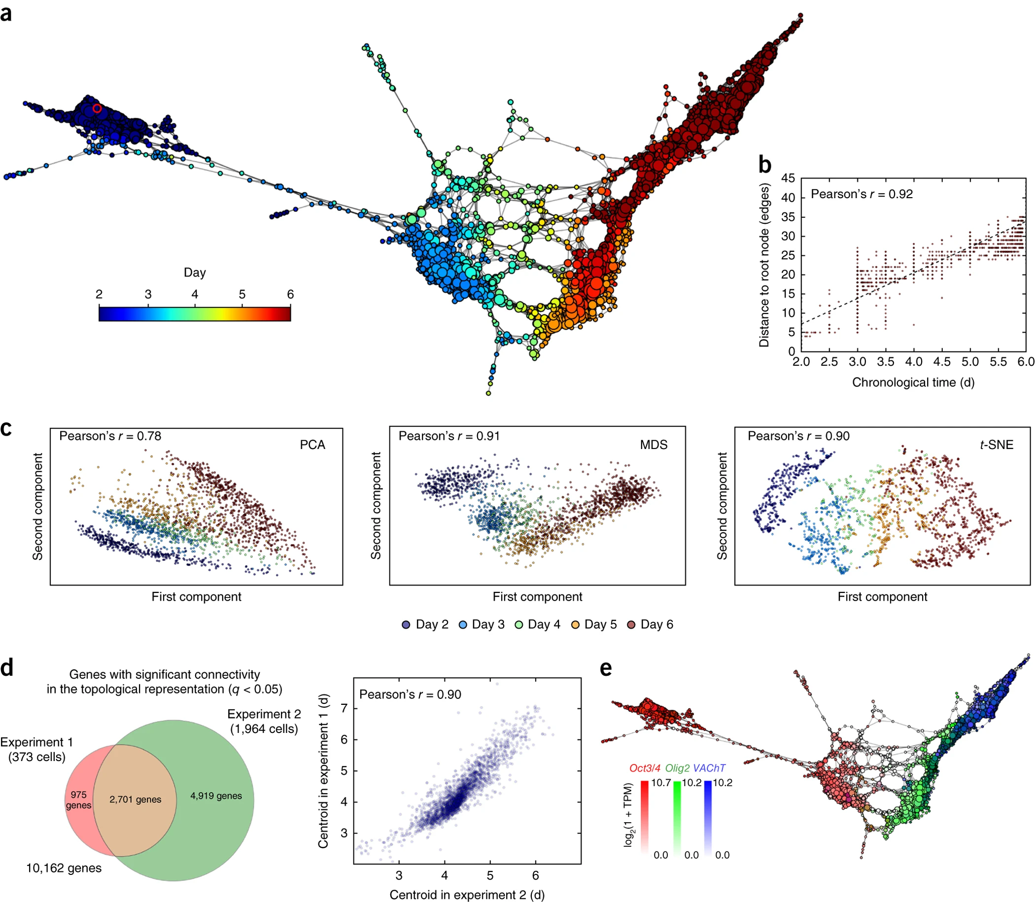 --- ## The shape of gene expression across plant evolution <p style="font-size: 9px; text-align: right; color: Grey;"> Credits: <a href="https://doi.org/10.1371/journal.pbio.3002397">Palande <em>et al.</em> (2023)</a></p> <div class="row"> <div class="column" style="max-width:42%"> <img style="padding: 0 0 0 0;" src="../../tda/figs/Mapper_ColorBy_Tissue.png"> <img style="padding: 0 0 0 0;" src="../../tda/figs/stress_leaf_lens.png"> </div> <div class="column" style="max-width:42%"> <img style="padding: 0 0 0 0;" src="../../tda/figs/tissue_leaf_lens.png"> <img style="padding: 0 0 0 0;" src="../../tda/figs/family_leaf_lens.png"> </div> </div> --- class: center, middle inverse # Case study ## Lung cancer <img src="../figs/amezquita_etal_2023.png" width="400" style="display: block; margin: auto;" /> --- # Setup - FPKM counts of RNAseq data from human lung tissue &rarr; 19,648 genes - 314 healthy samples (GTEx) - 500 cancerous samples (TCGA) - Considered Z-scores drawn from a Gaussian Mixture Model (GMM). - Perform a statistically accurate transformation from 2 to 1 Gaussian  --- # Filter function: mean correlation Compute the correlation of every patient with respect to every other patient - Each subject is assigned 813 values Then take the **mean correlation** value - Each subject is now assigned a **single** value 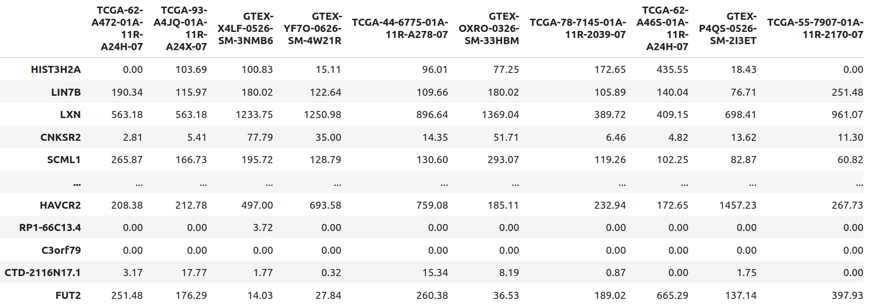 --- # Mapper setup - Filter by mean correlation (average of 814 correlation values) - Vary the number of bins `\(60 \leq b \leq 110\)` - Vary the overlap percentage `\(30 \leq p \leq 80\)` - Color the mapper node based on the number of healthy subjects in the cluster - Bright yellow: 100% cancerous samples - Deep purple: 100% healthy samples .pull-left[ 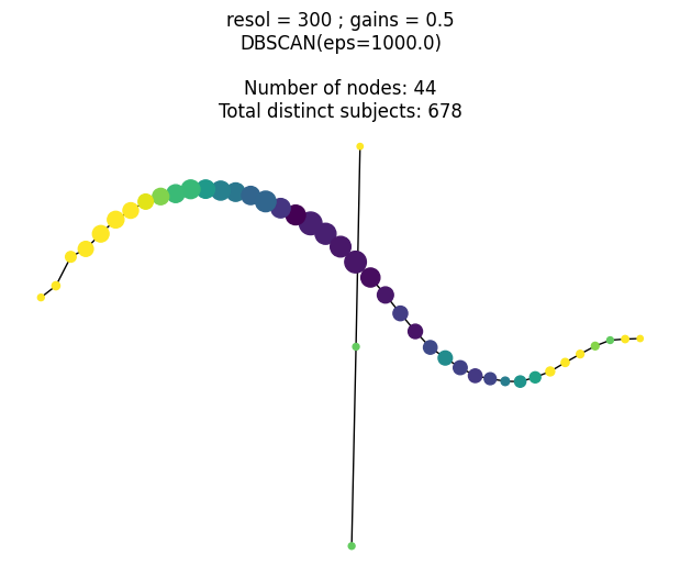 ] .pull-right[ 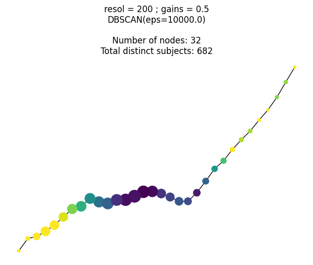 ] --- # Notice that cancerous samples are split .pull-left[   ] .pull-right[ - Mapper produced mostly strand-like graphs regardless of parameters used - Position Index for each subject: - **`-1`**: subject is part of the 13 leftmost nodes - **`+1`**: subject is part of the 13 rightmost nodes - Healthy subjects tend to stay at the center - Cancerous samples are distributed at both ends ] --- # This split cannot be captured with t-SNE! - tSNE does a pretty good job separating healthy vs cancerous samples (purple vs yellow) - However, finer structural details are lost - (a): Using FPKM - (b): Using GMM Z-scores  --- # Mathematical stability - When varying several parameters, the cancerous samples exhibit a much different behavior on the mapper graph than the healthy subjects. - Confidence intervals (black: superior limit, green: lower limit, red: average value) <img src="https://journals.plos.org/plosone/article/figure/image?size=large&id=10.1371/journal.pone.0284820.g010" width="500" style="display: block; margin: auto;" /> --- # Biological significance  --- # Future perspectives and Conclusions .pull-left[ Maintained python libraries to compute mapper - [Giotto-tda](https://github.com/giotto-ai/giotto-tda) - [KeplerMapper](https://kepler-mapper.scikit-tda.org/en/latest/)  Data visualization to inspire new research ] .pull-right[ Plenty of untapped potential in plant genomics  Agnostic to any kind of omics data ] --- background-image: url("https://upload.wikimedia.org/wikipedia/commons/4/4a/University_of_Missouri_logo.svg") background-size: 60px background-position: 99% 1% class: inverse # Thank you! <div class="row"> <div class="column" style="max-width:15%; font-size: 15px;"> <img style="padding: 0 0 0 0;" src="http://math.hawaii.edu/home/board/Farzana-Nasrin.jpg"></img> <p style="text-align: center;">Farzana<br>Nasrin (Hawaii)</p> </div> <div class="column" style="max-width:15%; font-size: 15px;"> <img style="padding: 0 0 0 0;" src="https://sites.lafayette.edu/storeyk/files/2022/01/ann_arbor_closer-e1641409616847.jpg"></img> <p style="text-align: center;">Katie<br>Storey (Lafayette)</p> </div> <div class="column" style="max-width:13.5%; font-size: 15px;"> <img style="padding: 0 0 0 0;" src="https://manoa.hawaii.edu/lifesciences/wp-content/uploads/sites/65/2021/09/MG_2781.jpeg"></img> <p style="text-align: center;">Masato<br>Yoshizawa (Hawaii)</p> </div> <div class="column" style="width:6.5%; font-size: 24px;"> <p></p> </div> <div class="column" style="max-width:50%; font-size: 24px; line-height:1.25"> <p style="text-align: center;"><strong>Email</strong></p> <p style="text-align: center; color: Blue; font-family: monospace;">eah4d@missouri.edu</p> <p style="text-align: center;"><strong>Website and slides</strong></p> <p style="text-align: center; color: Blue; font-family: monospace;">ejamezquita.github.io</p> </div> </div> <div class="row"> <div class="column" style="max-width:15%; font-size: 15px;"> <img style="padding: 0 0 0 0;" src="https://yt3.ggpht.com/a/AGF-l78XW3rduhw9ZYiOvZAQpKarAcON8RIQtnjd1A=s900-c-k-c0xffffffff-no-rj-mo"></img> <p style="text-align: center;">COBRE &mdash; P20GM125508</p> </div> <div class="column" style="max-width:12%; font-size: 15px;"> <img style="padding: 0 0 0 0;" src="https://news.brown.edu/sites/default/files/styles/vertical/public/article_images/ICERM_2.jpg?itok=5pmDGGSU"></img> </div> <div class="column" style="width:23%; font-size: 15px;"> <p> Vladislav Bukshtynov<br> Steven Ellis<br> Elin Farnell<br> Hwayeon Ryu<br> Sarah Tymochko </p> </div> <div class="column" style="max-width:50%; font-size: 24px; line-height:1.25"> <img style="padding: 0 0 0 0;" src="../figs/amezquita_etal_2023.png"> </div> </div> --- class: inverse, middle, center # Supplementary material --- ## Z-scores from a Gaussian Mixture Model (GMM) Let `\(y\)` be a random `\(p\)`-dimensional vector generated by a GMM of `\(K\)` components: `$$f(y) = \sum_{k=1}^K \pi_k\varphi(y | \mu_k, \Sigma_k)$$` - According to Bayes' Theorem, the posterior probability `\(w_k=P(c=k|y)\)` that `\(y\)` belongs to the `\(k\)`-th class is given by `$$w_k = \frac{\pi_k\varphi_k(y)}{\sum_{k=1}^K\pi_k\varphi_k(y)}$$` `$$T_0 = Z\cdot\mathbb{I}(\tilde{s}_1 = s_1) + (\tau^{-1}Z - \Delta_1)\cdot\mathbb{I}(\tilde{s}_1 > s_1) + (\tau Z + \tau\Delta_1)\cdot\mathbb{I}(\tilde{s}_1 < s_1)$$`