Day 11 Pre-Class Assignment

✅ Put your name here

¶

Computational Models Overview and The Pandas Data Analysis Library¶

Credits: Wikipedia

Learning goals for today’s assignment¶

• Review some types of Computational Models

• Use the Pandas module to explore and visualize data

Assignment instructions¶

Watch the videos below, do the readings linked to below the videos, and complete the assigned programming problems. Please get started early, and come to office hours if you have any questions! Make use of Slack as well!

This assignment is due by 11:59 p.m. the day before class, and should be uploaded into appropriate the “Pre-class assignments” submission folder. Submission instructions can be found at the end of the notebook.

Part 1: Overview of Computational Models¶

So far this semester, we looked and and even built a few examples of computational models. Take a moment to think about what we mean when we talk about “models” by watching the following overview video to get an introduction to the definition of Computational Models.

Note: This video references a model for the motion of a snowball. If you want to learn more about the model, ask your instructor!

✅  Question 1:

In your own words, decribe what scientific and/or computational models do.

✎ Put your answer here

✅  Question 2:

What are some of the limitations of scientific and/or computational models?

✎ Put your answer here

Part 2: Working with data in Pandas¶

Pandas is an extremely useful Python library for reading and analyzing datasets in a variety of formats with a variety of data types. Loading and managing complicated files with only the Python tools we’ve learned up to this point is often very difficult and at times, may seem impossible. Lucky for you, someone else decided to make your life easier and created Pandas!

Watch the following videos to learn a bit about how you can load and analyze data using this handy library! Pay particular attention to the part of the video that talks about “slicing” the data.

Note: In a previous semester of this course, the order of the topics covered was slightly different so there may be references to “future” content that you already have experience with. Also, the version of Python used in this video is a bit older than the version that you have, so the format of the Pandas dataframe might look a bit different in your notebook when you display it in your notebook.

Video 1¶

Video 2¶

This next video introduces plotting dataframes using the Pandas module. Pandas does have its own plotting functions which you may see referenced from time to time. You are welcome to explore them and use them, but in this course, we will focus on using Pandas (or NumPy) for loading and analyzing data and Matplotlib for visualizing the data! Matplotlib is a dedicated module for plotting, so it has much more flexibility and options.

Note: this video will reference the “blood pressure” dataset, which you will be working with in the code cells below.

Useful Pandas references¶

For this pre-class assignment and the assignments that follow during the next week of the course, these two references might prove to be particularly useful:

• The Pandas website

• 10-minute Pandas Tutorial

2.1: Loading data with Pandas¶

Now that we understand a bit of the fundamentals for Pandas dataframes, we’re going to use a small database of data taken from patients that were admitted to the hospital with chest pains. In the dataset, there are several columns. Here are what a few of them correspond to:

• age is patient age

• chol is serum cholesterol in units of mg/dl

• trestbps is the resting blood pressure of the patient upon admission

• thalach is the maximum heart rate achieved

The cell immediately below this uses Pandas to read in the data, and you should run that cell before you do anything else and make sure you understand what it’s doing!

Importing Pandas and all of our other useful modules we know up to this point.¶

As always, we should make sure we import all of the Python modules we might want to use as we work through the notebook.

Then, download heart_disease_data.csv from canvas. Make sure the file is in the same folder as your notebook! If you are having trouble with the data file, make sure to ask for help!

Pay special attention to the new import command for Pandas, it’s a bit different than what is shown in the video!

Make sure you execute this cell!

2.2: Checking out the DataFrame¶

Now let’s see what the data looks like by examining all of the columns labels and the first few rows of data using the .head() command that was explained in the video.

Let’s also test out the .describe() function to get some details about the data.

2.3: Accessing data in Pandas Dataframes (I)¶

To access data in a DataFrame for plotting, there are several different ways. Review the code below to see how you access data by its column header.

Note: In Part 3, we will explore additional ways to access data with more control!

To access the data by column name, you need to know the labels for each column name. If you need to know what strings pandas is using for column headers, you can find out using the .columns attribute (notice that there are no parentheses). Run the cell below to get the column header names for heart_disease_data.

Note: Using .columns is particularly useful when there are extra spaces or other attributes of the column names that you can’t see with the standard dataframe display. Remember this if you decide to use data for your semester project!

✅  Task 3

In the cell below, print another one of the columns of heart_disease_data

2.4 Visualizing the data¶

The following questions give you a chance to try visualizing the pandas dataframe using some of the functions you were shown in the video and one you weren’t.

Note: In this section, you will be plotting using the Axes interface of matplotlib. Remember that Axes is almost like using the pyplot interface shown in Video 2.

✅  Task 4:

• Using plt.subplots, make a histogram (using ax.hist()) of the resting blood pressure of the patient upon admission.

• Make sure to include axis labels and a title indicating what you’re looking at.

✅  Task 5:

• Make a scatter plot of the resting blood pressure ('trestbps') versus age. Make sure you put the right variables on the x- and y-axes.

Think back to (or refer to) the mass-to-femur in-class assignment we did last to remind yourself about correlations. Do you think these values are correlated?

✅  Task 6:

• Make a boxplot for the resting blood pressure.

• Add a grid (ax.grid) to your plot

Like ax.hist, the code structure of ax.boxplot is slightly different than ax.plot or ax.scatter because it contains only one dimension of data (i.e. one column of a dataframe).

✅  Question: 7

Reading the boxplot.

• What does the box actually represent?

• What is the meaning of the orange line in the middle of the box?

• What about the circles that are floating atop?

You can read more about boxplots in Wikipedia and matplotlib.

Part 3: Accessing Parts of Dataframes¶

What if we want to access dataframes by something other than the column headers?

✅  Task 8:

The three cells of code below creates a dataframe from scratch and manipulate it.

• Review the code and, when necessary, use the internet to learn what the following Pandas methods/attributes are used for (e.g. .index and .columns)

• Comment on what each line of code is doing below.

Now that we’ve created this Pandas dataframe, the following image should serve as a reference for how one can access information within it.

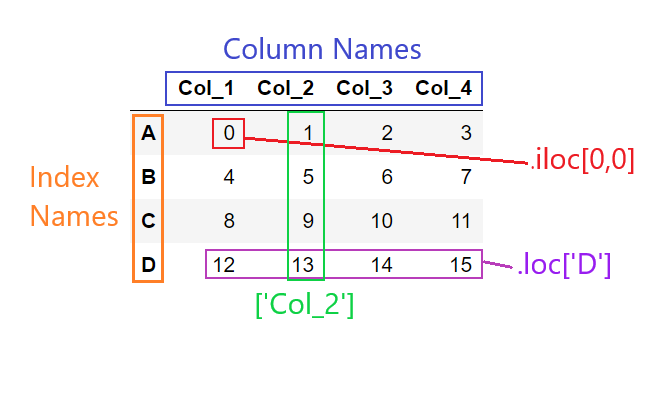
3.1: Examples of using .iloc and .loc to access data¶

Have you figured out the difference yet?

• If you want to access data by its label or name, we use .loc

• If you want to access data by its indices or position, we use .iloc

Now, here are some examples that require us to index Pandas dataframes:

✅  Example 1:

Access information in the second column of example_dataframe.

• Information Needed: Look at the above image and in your mind ‘highlight’ the information we want to access. We want the values under Col_2.

• Available Tools:

  • We notice that since we want all the information in the column, we can access it by the column name.

  • However, we can also simply retreive the values in that column using .iloc. We want all the rows in the column at the 1 index.

Check your code: Look at the gif below. Is this the image you pictured earlier? We can check that the code we used was correct by comparing the output with the column highlighted in the original dataframe.

✅  Example 2:

We access the information in the second row in a similar manner.

Now, we have a slightly more complicated task. We are going to access single entries or multiple entries in a single column.

✅  Example 3:

Access the top left element of the example_dataframe.

• Information Needed: Look at example_dataframe and in your mind ‘highlight’ the information we want to access. We want the value 0.

• Available Tools:

  • Since we want a single value, we can combine the column and row access we used before, by using both the column name and .loc with the row name.

  • Or we could use the indices to retreive the value using .iloc. We want the entry in the 0th row and 0th column.

We can also access multiples entries. In the final example, we want to access the entries 1,2,3 or the entries in the 0th row and the 1st, 2nd, 3rd columns.

Check your code: Look at the gif below. We can check that the code we used was correct, by comparing the output with the column highlighted in the original dataframe.

3.2: Let’s practice different ways to index using both .iloc and .loc¶

Examine the Example_Dataframe and complete the questions below. For each question, follow the same process we did above: What is the task? What information do you need? What tools can you use? Make sure to check that the output matches what you expected from the original Dataframe. For the Available Tools portion in Tasks 1 and 3, make sure to describe the differences between the two methods.

✅  Task 9:

Using .loc and .iloc, access and print the row of data containing [8,9,10,11] from the example dataframe.

• Information Needed:??

• Available Tools:

  • ??

  • ??

✅  Task 10:

Using .iloc, access and print just the values [6,10,14] from the example dataframe.

• Information Needed:??

• Available Tools:

  • ??

✅  Task 11:

Using .loc and .iloc, access and print the value 10 from the example dataframe.

• Information Needed:??

• Available Tools:

  • ??

  • ??

✅  Task 12:

Print out the column names and index names of the example dataframe.

3.3: Understanding the Pandas Dataframes default¶

By default, when you load a dataset with Pandas or create a dataframe from scratch, Pandas will define the row indices to just be numbers rather than a unique set of labels that match your data. This is how we will commonly interact with Pandas dataframes.

✅  Task 13

• Review the following code that constructs a dataframe without providing specific row index names

• Comment what each line of code is doing.

Indexing will be similiar to before but now the row names are just integers representing row numbers.

Congratulations, you’re done!¶

Submit this assignment by uploading it to the course Canvas web page. Go to the “Pre-class assignments” folder, find the appropriate submission folder link, and upload it there.

See you in class!

Material drawn with permission from:
© Copyright 2023. Department of Computational Mathematics, Science and Engineering at Michigan State University

Adapted for:
© Copyright 2026, Division of Plant Science & Technology—University of Missouri