Day 17 Pre-Class Assignment

✅ Put your name here
¶

Hypothesis testing, standard errors, and bootstrapping¶

Comic about hypothesizing how hypothesis come to be.

Learning goals for today’s pre-class assignment¶

State what hypothesis testing is and how to interpret a null hypothesis.
Compute and interpret correctly standard errors.
List the steps of a bootstrap procedure and relate the results to the standard error.

Assignment instructions¶

This assignment is due by 11:59 p.m. the day before class, and should be uploaded into the appropriate “Pre-class assignments” submission folder. If you run into issues with your code, make sure to use Slack to help each other out and receive some assistance from the instructors. Submission instructions can be found at the end of the notebook.

1. Hypothesis testing and the null hypothesis¶

You may not realize it, but in the past few days you have been stating null hypotheses, computing adequate statistics to test such hypotheses, alongside associated p-values. For example in last class, when you computed the Pearson correlation between oil and protein content in soybeans, you posed the null hypothesis:

There is no linear correlation between the oil and the protein content in soybean.

The adequate statistic to determine whether such hypothesis is likely or not is Pearson’s $r$ correlation coefficient. In this case, we got $r = 0.72$ .

Remember that the p-value means that “the probability of getting such $r$ value due to sheer chance”. We got a p-value $<2.2\times10^{-16}$ , so our high $r$ value is very much not a fluke.

And so—considering the $r$ , the $p$ , AND the scatterplot—we can reject the null hypothesis. In other words, there it is very likely that there is indeed a correlation between oil and protein contents.

IMPORTANT: NO statistical test will ever tell you unequivocally if a null hypothesis is true or not. It will rather tell you how likely is for the hypothesis to be true based off the data you provided the test. This is an important distinction. If your data is biased or does not meet the test conditions, then the test results will be biased or incorrect. Failing to understand this distinction is what often times leads to bad science.

This is why it is important to always support your statistical numbers with proper visualization.

1.1 Rejecting vs failing to reject¶

Null hypotheses are not limited to correlations.

Watch the following video on what is hypothesis testing and a null hypothesis in general. Keep in mind the hypotheses posed regarding Drugs A, B, C, D, E, and F.

from IPython.display import YouTubeVideo
YouTubeVideo("0oc49DyA3hU",width=640,height=360)

✅ Question 1

Consider the first hypothesis along its (carefully conducted) experiment results from the video:

People taking Drug A need, on average, 15 fewer hours to recover than people taking Drug B.

Are the following two statements the same? Based off the experiment results...

...we can reject the hypothesis.
...the hypothesis is likely false.

Explain your answer.

✎ Put your answer here.

✅ Question 2

Consider the second hypothesis along its (carefully conducted) experiment results from the video:

People taking Drug C need, on average, 13 fewer hours to recover than people taking Drug D.

Are the following two statements the same? Based off the experiment results...

...we fail to reject the hypothesis.
...the hypothesis is likely true.

Explain your answer.

✎ Put your answers here.

✅ Question 3

Consider the third hypothesis along its (carefully conducted) experiment results from the video:

There is no difference in recovery times between Drug E and Drug F.

Are the following two statements the same? Based off the experiment results...

...we fail to reject the hypothesis.
...the hypothesis is likely true.

Explain your answer.

✎ Put your answer here.

1.2 Practicing with previous examples¶

Let’s revisit the results from Figure 3 from Kettenbach et al (2024) which we discussed back in in-class day 15.

Julian day of collection for flowering Polemonium and Salix as a function of average daily low temperature in June of the collection year.

Credits: Kettenbach et al (2017)

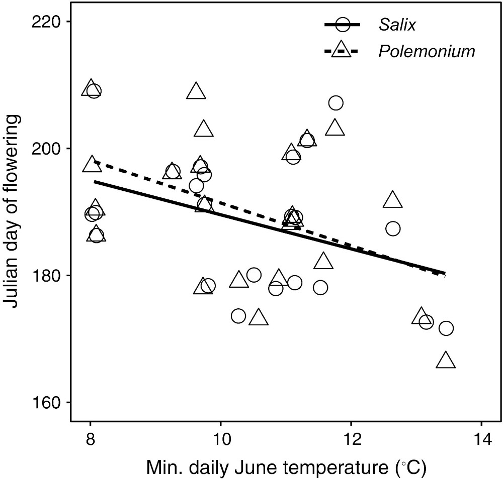
Julian day of collection for flowering Polemonium and Salix as a function of average daily low temperature in June of the collection year. Open circles and solid line show data for Salix while triangular symbols, and dashed line show data for Polemonium ( $y = 228 - 3.7x$ ) and $y = 235−4.3x$ ; respectively).

✅ Question 4

Back in In-Class 15 (Part 4), we computed the Pearson correlation coefficient between flowering time and temperature.

For Polemonium
The Pearson coefficient is -0.52
Its associated p-value is 0.009

For Salix
The Pearson coefficient is -0.48
Its associated p-value is 0.017

In Polemonium ans Salix terms, what are the two null hypotheses that we are testing for in Figure 2? (One for each plant species).

✎ Put your two answers here.

✅ Question 5

Based off the scatterplot alone, do you reject or fail to reject each of the null hypothesis you proposed for Question 4?

Give two answers, one per null hypothesis.

✎ Put your two answers here.

2. Standard error of the mean¶

Correlations are not the only sorts of null hypotheses we can pose. In the next few weeks, we’ll focus on two-sample tests, where we pose questions like in the first video:

There is no difference between the means of these two samples (control vs. treatment, male vs. female, wild type vs. mutant, etc.)

But in that case, we need to have a sense of how much the mean can vary, what is the error when measuring our sample mean.

2.1 The intuition and the formula¶

Watch the first 8:45 mins of this video that explains the meaning of the “standard error of the mean”

YouTubeVideo("XNgt7F6FqDU",width=640,height=360, stop=8*60+45)

✅ Question 6

In your own words, what is the difference between standard deviation and standard error?

✎ Put your answer here.

The StatQuest above does mention that there is a formula for the standard error but does not state it. The actual formula—which is what pandas and SciPy use—is:

\text{Standard Error} = \frac{\text{Standard Deviation}}{\sqrt N}.

(1)

Where $N$ is the number of sample points we have.

Important: The formula above uses the Standard Deviation of the total population. However, we almost never have measurements for the total population. We just have a sample, and based on that sample we estimate the standard deviation. In that case, the formula above will give us an estimate of the standard error rather than the actual value.

2.2 Looking at an example¶

Let’s stick to the Kettenbach et al (2024) data. This time we turn to Figure 5 and contaminated pollen: the proportion of Salix (invasive) pollen found on Polemonium (native) flowers across different locations and altitudes in Colorado. The locations are Hoosier East (HE), Hoosier West (HW), and Weston Pass (WP).

Import the usual modules
Load the data and drop NaNs

# Import modules and load the data

import pandas as pd
import matplotlib.pyplot as plt
import numpy as np
from scipy import stats

data = pd.read_csv('2016+population+survey.csv').dropna(axis=0, how='any')
print(data.shape)
data.head()

(120, 7)

Let’s focus just on the pollen contamination values for Polemonium collected at Weston Pass
Remember that we can use .loc and mask to get a Series

site = 'Weston Pass'
contamination = data.loc[data['site'] == site, 'frequency of Salix pollen']
contamination.head()

30    0.025974
31    0.010101
32    0.009346
33    0.008511
34    0.109375
Name: frequency of Salix pollen, dtype: float64

Since we have a Series, we can use pandas .sem function to compute it standard error of the mean.
- This works only if we are dealing with DataFrames or Series, which is the most common thing to be working with
Alternatively, stats also has a .sem function that also works with lists or arrays.
Or we can compute the formula “by hand” with NumPy.

# SE with pandas
print('Standard Error with pandas:\t', contamination.sem())

# SE with stats
print('Standard Error with stats:\t', stats.sem(contamination))

# SE with formula and NumPy
print('Standard Error with NumPy:\t', np.std(contamination, ddof=1)/(len(contamination)**0.5))

Standard Error with pandas:	 0.01088565889298954
Standard Error with stats:	 0.01088565889298954
Standard Error with NumPy:	 0.01088565889298954

✅ Task 7 (optional)

Compute the standard error—however you like—for pollen contamination at Pennsylvania Mountain.

# Your code

3. Bootstrapping¶

3.1 How to make multiple samples out of a single sample¶

Finally, watch the rest of the last video which quickly goes into bootstrapping.

YouTubeVideo("XNgt7F6FqDU",width=640,height=360, start=8*60+44)

✅ Question 8

In your own words, describe the six steps to compute the standard error when “bootstraping your data”.

✎ Put your answer here.

3.2 Bootstrapping an example¶

Resampling involves reusing your one dataset many times. It almost seems too good to be true! In fact, the term "bootstrapping" comes from the impossible phrase of pulling yourself up by your own bootstraps! However, using the power of computers to randomly resample your one dataset to create thousands of simulated datasets produces meaningful results.

Let’s again focus on contaminated pollen from Weston Pass.
Like StatQuest, let’s plot all those values on a horizontal line and draw a vertical line for the mean.

# StatQuest-like plot of our root weight values

fig, ax = plt.subplots(figsize=(10,1))
ax.set_ylim(-0.3, 0.3)
ax.set_yticks([0], '')
ax.set_title(site)
ax.set_xlabel('Pollen contamination %')
ax.axhline(0, c='k', lw=2, zorder=1)
ax.plot([contamination.mean(), contamination.mean()], [0.2, -0.2], c='r', lw=3, zorder=2)
ax.scatter(contamination , np.zeros(len(contamination)), marker='o', s=100, fc='r', ec = 'k', zorder=3);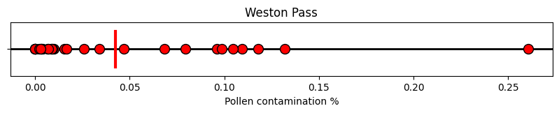

With NumPy’s random generator and rng.choice, we can resample our data as many times as we want. Say we resample 10 times. Just like StatQuest, we plot every sample in a horizontal line and indicate its mean.

# random number generator
rng = np.random.default_rng(seed = 42)

# Number of resamples for bootstrap
N = 10

# Plot code
fig, ax = plt.subplots(figsize=(10,2.5))
ax.set_ylim(-1.75, 0.3)
ax.set_yticks([0], '')
ax.set_title(site)
ax.set_xlabel('Pollen contamination %')
ax.axhline(0, c='k', lw=2, zorder=1)
ax.plot([contamination.mean(), contamination.mean()], [0.2, -0.2], c='r', lw=3, zorder=2)
ax.scatter(contamination , np.zeros(len(contamination)), marker='o', s=100, fc='r', ec = 'k', zorder=3)

means = np.zeros(N)

for i in range(N):
    sample = rng.choice(contamination, size = len(contamination), replace=True) # Resample allowing replacements
    means[i] = sample.mean() # Save the mean of the resample

    nudge = -0.15*(i+1) # Every resample will be plotted a nudge below the previous one

    plt.axhline(nudge, c='gray', ls='dashed', lw=1, zorder=1)
    plt.scatter(sample , nudge+np.zeros(len(contamination)), marker='d', s=50, fc='dodgerblue', ec = 'k', zorder=2)
    plt.plot([means[i], means[i]], [nudge+0.1, nudge-0.1], c='blue', lw=3, zorder=3)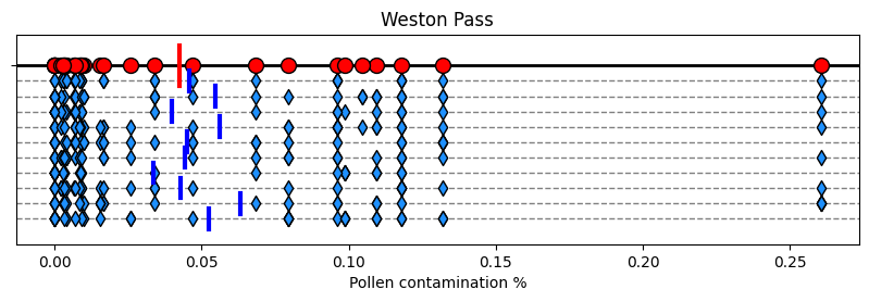

Like in StatQuest, the bootstrapped means (in blue) are not that faraway from the true mean (in red). Remember that the standard error is the standard deviation of the means. So we compute exactly that:

Sidenote: The ddof=1 tell NumPy to divide the variance by N-1 instead of N. You don’t need to worry about it at the moment, but you can watch another StatQuest on why this is necessary when you have small samples if you’re curious.

# Standard deviations from the mean
means.std(ddof=1)

0.008799369005180328

We see that 0.0088 is fairly close to the formula value we got before of 0.0109. Can we get a closer estimate? Let’s increase our sample to number to 10000!

# random number generator
rng = np.random.default_rng(seed = 42)

# Number of resamples for bootstrap
N = 10000
means = np.zeros(N)

for i in range(N):
    sample = rng.choice(contamination, size = len(contamination), replace=True) # Resample allowing replacements
    means[i] = sample.mean() # Save the mean of the resample

print('The standard deviation of',N,'bootstrapped samples is',means.std(ddof=1))

The standard deviation of 10000 bootstrapped samples is 0.010714403086510726

By taking 10,000 resamples, our standard error estimate is 0.0107 which is fairly close to 0.0109. Yay.

You can take an even larger number of resamples but your estimate might not improve.

Important: Bootstrapping is just as good as the number of samples from your original experiment. In this case, having 20 original datapoints is just good enough. But if we only had 5 datapoints, we would see a larger discrepancy between the formula and bootstrap standard errors.

✅ Task 9

Make sure you understand what all the code above is doing. Read especially the documentation of the rng.choice function that we use to resample an original array/Series.

✅ Task 10

Remember that the standard error is “the standard deviation of the means taken for multiple samples from the same population.” The formula for standard error of the mean— $\text{SE} = \text{SD}/\sqrt N$ —is exact only when we have the exact standard deviation of the population, which is almost never the case in real life. We only have the an estimation of the standard deviation using one sample of Polemonium flowers.

With all that in mind: which value do you think is closer to the true Standard Error?

0.0107, estimated with bootstrap?
0.0109, estimated with the SE formula?

Explain your answer.

✎ Put your answer here.

3.3 Alternatively, we can use `stats.bootstrap`¶

Above we have computed lots and lots of bootstrapped samples based off our original 20 datapoints. Ulitimately, we only care about the standard deviation of the mean. We don’t really care about the bootstrapped samples themselves—the blue diamonds and blue bars.

In that case, we can use the stats.bootstrap function to do most of the work for us. You will notice that it runs much faster than our manual implementation.

# random number generator
rng = np.random.default_rng(seed = 42)

# Compute the bootstrap
# - The input data `contamination` must be in a single sequence: we do that by making it part of a tuple of length 1
#   - Notice the comma INSIDE the parentheses
# - We are interested in the standard deviation of what statistic?
#   - The function to compute the mean is `np.mean`
# - Specify the number of resamples
# - Specify the random number generator for reproducibility

boot = stats.bootstrap( (contamination,), statistic=np.mean, n_resamples=N, rng=rng)

# `boot` is a named tuple, just like when we compute correlations or linear regressions
print('The standard deviation of',N,'bootstrapped samples is', boot.standard_error)

The standard deviation of 10000 bootstrapped samples is 0.010714403086510726

We indeed get the same result compared to our manual bootstrap above. This is because in both cases we used the exact same random number generator.

✅ Question 11

Compare and contrast the code for a manual bootstrap and the code for stats.bootstrap.

Which option seems easier to use to you?

✎ Put your answer here.

✅ Task 12

For the contamination sample, use bootstrap—whichever way you prefer— to compute its standard error of the median.
That is, the standard deviation of medians taken from $N = 10000$ samples.

Note: There is no nice formula for standard error of the median. But bootstrap does not care about that and still gets us a good answer.

# Your code

Congratulations, you’re done!¶

Submit this assignment by uploading it to the course Canvas web page. Go to the “Pre-class assignments” folder, find the appropriate submission folder link, and upload it there.

See you in class!

References¶

Kettenbach, J. A., Miller‐Struttmann, N., Moffett, Z., & Galen, C. (2017). How shrub encroachment under climate change could threaten pollination services for alpine wildflowers: A case study using the alpine skypilot,Polemonium viscosum. Ecology and Evolution, 7(17), 6963–6971. 10.1002/ece3.3272

✅ Put your name here¶

Hypothesis testing, standard errors, and bootstrapping¶

Learning goals for today’s pre-class assignment¶

Assignment instructions¶

1. Hypothesis testing and the null hypothesis¶

1.1 Rejecting vs failing to reject¶

1.2 Practicing with previous examples¶

2. Standard error of the mean¶

2.1 The intuition and the formula¶

2.2 Looking at an example¶

3. Bootstrapping¶

3.1 How to make multiple samples out of a single sample¶

3.2 Bootstrapping an example¶

3.3 Alternatively, we can use stats.bootstrap¶

Congratulations, you’re done!¶

✅ Put your name here
¶

3.3 Alternatively, we can use `stats.bootstrap`¶