Are oil and protein contents related in soybean cultivars?
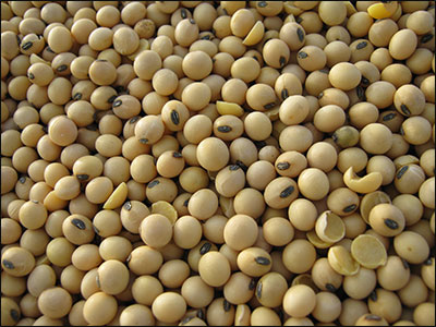
Credits: MU Variety Testing Program
Learning goals of today’s assignment
Practice fitting linear models with SciPy.
Assess how good is the linear model in the first place.
Use your model to predict oil and protein content for other soybean cultivars.
Assignment instructions
Work with your group to complete this assignment. Instructions for submitting this assignment are at the end of the notebook. The assignment is due at the end of class.
Background
Soybean is currently promoted in sub-Saharan Africa as a high-quality protein source. Breeding soybean for improved seed composition requires understanding how cultivars interact with these new environments. This study evaluated genotype by environment interactions and the genetic diversity of cultivars grown in the Pan-African Soybean Variety Trials (PATs). They identified cultivars with increased protein or oil in specific environments or stable performance across environments. Their results provide valuable resources for improving soybean seed composition in sub-Saharan Africa. Work supported by USAID’s Feed the Future Soybean Innovation Lab and by the University of Missouri Northern Soybean Breeding Program.
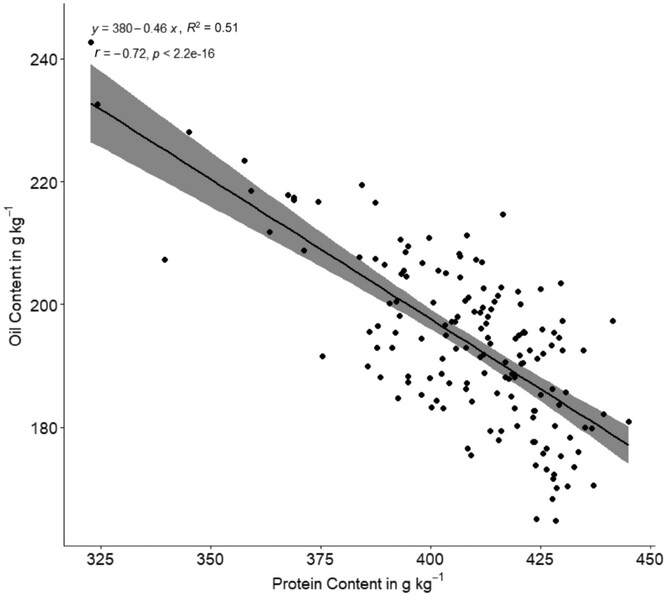
Credits: De Meyer et al (2024)
More details in:
De Meyer, E., Prenger, E., Mahmood, A., da Fonseca Santos, M., Chigeza, G., Song, Q., Mwadzingeni, L., Mukaro, R., Chibanda, M., Mabuyaye, G., Diers, B., & Scaboo, A. (2024) Evaluating genetic diversity and seed composition stability within Pan-African Soybean Variety Trials. Crop Science, 64, 3272–3292.
✅ Question 1
In your own words, what information do you get out of this figure?
✎ Put your answer here
1. Setting everything up
Before jumping straight into linear regressions, we need to go through the usual setup steps.
✅ Task 2
Import the usual suspects: NumPy, pandas, matplotlib, and Scipy’s stats
# Remember that it is always good coding practice to import your libraries at the top before doing anything else.
# Import the rest of modules

import numpy as np
✅ Task 3
With pandas, load the dataset
PATSA_final_QCd_rep_data.csvas a variabledataDrop all the pesky rows with NaNs.
Display its first few rows to make sure everything worked as expected.
# Load the data

# data = ???
# data = data without NaNs
# data
✅ Question 4
What columns will you need to reproduce Fig. 2 from De Meyer et al. (2024) (the figure displayed in Background)?
✎ Put your answer here.
✅ Task 5
With matplotlib, make a scatterplot of oil vs protein content for all the samples in the data.
Make sure to label your axes
You’ll notice that your scatterplot and regression values are a bit different from the one published by De Meyer et al. We’ll fix that later.
# Your plot

# fig, ax =
# scatterplot ( protein , oil , ... )
# axes labels and titles
✅ Task 6
With
stats.pearsonr, compute and print the Pearson correlation between oil and protein content and its associated p-valueUse the dot
.and name to access these values. Do NOT use indices.
# Pearson correlation✅ Question 7
Looking at both the plot, the correlation coefficient, and its p-value, do you think that oil and protein content are correlated?
If so, do you think it makes sense to fit a linear model?
✎ Put your answer here.
2. Predicting values with linear regression and stats.linregress
Now it is your turn to compute linear regressions as in the Pre-Class
✅ Task 8
Compute a linear regression between protein and oil soybean content. Remember that order matters!
Is your reported linear formula close to the one reported by De Meyer et al (2024)?
Make sure you use the dot
.and name to access these regression values. Do NOT use indices.
# Your regression✅ Question 9
Based solely on the slope and intercept values:
How many grams does oil content increase (or decrease) for every protein gram gained by the soybean?
Theoretically speaking, what is the maximum possible oil content a soybean can ever achieve?
✎ Put your answer here.
✅ Task 10: Predicting Values
Based on you linear model:
What would be the oil content of a soybean cultivar with 500g of protein? 250g?
# Write some code to answer the two questions✅ Task 11
Now plot the actual best-fit line. You can either:
Define a
pred_proteinarray with sensible start and end points; then use it to predict an arraypred_oilof oil values (Method #1).
or
Use the
.axlinefunction (Method #2).
# Copy/paste your code from T5 here
# fig, ax =
# scatterplot ( protein , oil , ... )
# axes labels and titles

# Method #1
# pred_protein = np.linspace( ... )
# pred_oil     = ...
# ax.plot( ... );

# Method #2
# xy1 = ( ... , ... )
# ax.axline( ... );
✅ Question 12
Compare the linregress reported values on Peason’s correlation coefficient and p-value versus those reported by pearsonr
Are they the same. Just type YES/NO
The cool thing of linregress is that it computes correlation at the same time!
✎ Put your answer here.
✅ Task 13: the other way around
Based on your drawn linear model:
What would be the protein content of a soybean cultivar with 150g of oil?
What is the theoretical limit of protein content for a soybean?
Remember that the inverted formula for is
# Write some code to answer the questions above
# inv_slope =
# inv_intercept =

# predict values
3. to assess goodness-of-fit (using with sklearn.metrics.r2_score)
We have computed a linear model, but how much does that model actually tell us? Remember that the score tells us how much of the -axis variance is explained by the -axis. And you guessed it, Python can compute the score for us! While you don’t need to remember the formulas (because Python does it for us) it is crucial that you know how to interpret the results.
To do the computations, we need to import the submodule metrics from the module Scikit-Learn. Scikit-Learn is Python’s main module to do anything machine learning related and more! This semester we will not delve into it, but it will be a recurring friend in the next course (just saying 😉.)
In this case, we want to know how much of the oil content in a soybean can be explained by its protein content.
✅ Task 15
Make a variable
oil_predwith the predicted oil content values for the actual protein content values. That is, the protein values that come from the dataset itself.Then compute the score of the linear model with
metrics.r2_score.
Important: the order of the arguments does matter! Read more about the function here.
# import the necessary submodule
from sklearn import metrics

# compute the R2 score
# oil_pred = something something data['PROTEIN_g/kg']
# metrics.r2_score(...)
4. Averaging values: wrangling practice
As mentioned earlier, the regression values are a bit off compared to DeMeyer et al (2024). That is because the paper considers averages across genotype and environment. In the raw data we’re using, we’re considering replicates. Let’s fix it!
4.1 Reminder: Pandas, .loc, and masking
During the pre and in-class 12 we went through masking. As a quick reminder
# To get all the rows where a column matches a value
data[ data['column name'] == value ]

# To get all the rows where two columns match two values
data[ (data['column name 1'] == value1) & (data['column name 2'] == value2) ]

# And so on and so forth

# To get all the rows where one OR two columns match one OR two values
data[ (data['column name 1'] == value1) | (data['column name 2'] == value2) ]
# Notice that `&` means AND, while `|` means OR
We can combine masking with .loc to just get specific column(s) instead:
# get a column where two other columns match two values
data.loc[ (data['column name 1'] == value1) & (data['column name 2'] == value2) , 'column name 3' ]
✅ Task 15
With the
genandenvvariables below, get the protein content of all the samples from Bimha genotype grown in environment Type 1.Then use
.mean()to compute the mean protein content
# Mask and .loc practice
gen = 'BIMHA'
env = 'ENV1'

# finish the code
We can also keep a summary of all the means for all the genotype-environment combinations. This summary can be a dataframe. Its entries are written with .loc.
✅ Task 16
Comment every line of the code below
If you are unsure what a line does, copy/paste it in another cell and print its contents
Also duckduckgo for documentation
Compare the values in the DataFrame with those in Figure 3a from De Meyer et al (2024).
# Run the cell and Comment every line below

genotypes = data['GEN'].unique()
environments = data['ENV'].unique()
print(genotypes, environments, sep='\n\n')

protein = pd.DataFrame(0., index=genotypes, columns=environments)
for gen in protein.index:
    for env in protein.columns:
        protein.loc[gen, env] = data.loc[ (data['GEN'] == gen) & (data['ENV'] == env) , 'PROTEIN_g/kg'].mean()

mean_protein = protein.to_numpy().flatten()
protein
---------------------------------------------------------------------------
NameError Traceback (most recent call last)
Cell In[11], line 3
1 # Run the cell and Comment every line below
----> 3 genotypes = data['GEN'].unique()
4 environments = data['ENV'].unique()
5 print(genotypes, environments, sep='\n\n')
NameError: name 'data' is not defined✅ Task 17
Make a summary dataframe
oiland its flattened arraymean_oilfor average oil content across genotypes and environments.You can either copy/paste the code above and edit; or simply add a few lines to the existing code
# 5. Recomputing the model
Now that we have average protein and oil content, let’s reproduce that actual De Meyer et al (2024) values. You’ll just need to copy paste your code from above and edit accordingly.
✅ Task 18
Using mean_protein and mean_oil arrays:
Compute the best-fit line and print the model values
Print the correlation coefficient, its p-value, and the score
Make a scatter plot of oil vs protein content and the best-fit line.
# Your code

# best-fit line between the mean protein and mean oil values
# oil_pred = something with the mean protein values
# R2 score between the mean oil values and oil_pred

# Make a plot
# fig, ax =
# scatterplot ( mean protein values, mean oil values, ... )
# axes labels and titles

# Method #1
# pred_protein = np.linspace( ... )
# pred_oil     = ...
# ax.plot( ... );

# Method #2
# xy1 = ( ... , ... )
# ax.axline( ... );
Congratulations, you’re done!
Submit this assignment by uploading it to the course Canvas web page. Go to the “In-class assignments” folder, find the appropriate submission link, and upload it there.
See you next class!
© Copyright 2026, Division of Plant Science & Technology—University of Missouri
- De Meyer, E., Prenger, E., Mahmood, A., da Fonseca Santos, M., Chigeza, G., Song, Q., Mwadzingeni, L., Mukaro, R., Chibanda, M., Mabuyaye, G., Diers, B., & Scaboo, A. (2024). Evaluating genetic diversity and seed composition stability within Pan‐African Soybean Variety Trials. Crop Science, 64(6), 3272–3292. 10.1002/csc2.21356