Day 23 Pre-Class Assignment

✅ Put your name here
¶

Multiple testing and comparisons¶

In statistics, a confounding variable is a third variable that's related to the independent variable, and also causally related to the dependent variable.

Learning goals for today’s pre-class assignment¶

Recognize the difference of a priori and post-hoc tests and know when to use which
State different options of post hoc tests and tell when one is preferrable over another

Assignment instructions¶

This assignment is due by 11:59 p.m. the day before class, and should be uploaded into the appropriate “Pre-class assignments” submission folder. If you run into issues with your code, make sure to use Slack to help each other out and receive some assistance from the instructors. Submission instructions can be found at the end of the notebook.

Make all the needed imports before anything else¶

import numpy as np
import pandas as pd
from scipy import stats
from matplotlib import pyplot as plt
from IPython.display import YouTubeVideo

We will make jitterplots across the assignment (and other plots), so it is good idea to define some variables from the the get-go

# Random noise for the jitterplots
rng = np.random.default_rng(seed = 42)
nudge = rng.uniform(-0.15, 0.15, 1000)

# Lists of colors and markers
colors = ["#a1dab4", "#41b6c4", "#2c7fb8", "#253494", "#ffffcc"]
markers = ['o', '^', 's', 'D', 'v']

# fontsize for all the plots
fs = 12

Multiple sample testing¶

So far, whenever we have multiple samples—multiple water temperatures or multiple switchgrass genotypes— we have compared each possible pair using two-sample tests like Welch’s and Mann-Whitney. We then adjust the p-values with Bonferroni or Benjamini-Hochberg (False Discovery Rate). The reason of why we adjust is because Welch’s or Mann-Whintey is oblivious to additional samples and additional tests being performed.

But, can we look at all the samples and all their differences at once? Can we make Welch or Mann-Whitney aware that there is extra stuff to consider so there is no need to adjust later?

Yes we can!

1. ANOVAs and omnibus tests¶

The first such test is the ANOVA (Analysis of Variance). Tests that take into account more than two samples at once are usually referred to as omnibus tests.

Watch the video below to learn more about ANOVAs (also known as F-tests).

Important: Do not worry too much about the math discussed across the video. ANOVA itself is outdated—but still taught due to the same inertia I ranted about in the last class. There are much more powerful alternatives readily available in Python.

However, ANOVAs are a good entry point to the whole omnibus vs post hoc discussion we’ll have below.

YouTubeVideo("mOdYddj5IG8",width=640,height=360)

1.1 Recaping ANOVAs and nominal variables¶

To recap, ANOVAs (F-tests) pose the null hypothesis (similar to t-tests):

There is no difference between the means of all the given samples

Following the examples from the video, ANOVAs help us analyze the variance by posing questions like:

Can variance in plant growth be explained by differences in fertizer.

Can variance in blood pressure be explained by differences in medication.

For the analyses above to be meaningful, we assume that the population being tested is identical except for the independent (nominal) variable. When dealing with fertilizer and plant growth, we assume that water, soil type, light availability, etc. are all the same for all the plants and the only thing that changes is the actual fertilizer being used.

But what if we vary two variables, like fertilizer and cover crop? That’s where two-way ANOVAs come into play. We will not talk much about two-way ANOVAS in this course.
But what if my data is noisy/it has more than two varying features? That’s where MANOVAs (Multivariate ANOVAs) come into play. We will not talk much about MANOVAs either.

1.2 Post hoc tests¶

In case you missed the very last part of the video above: Consider the blood pressure experiment from the video, where we have three drugs A, B, and C.

An small p-value ANOVA suggests that not all treatment groups are the same. However, it does not tell you which groups might not be the same. That is where post hoc tests come into play. Tests that we do after (post) ANOVA.

The crudest post hoc test would be to do three two-sample tests:

A vs B
A vs C
B vs C

And then adjust their p-values for false positives (like we discussed in Day 24 with Benjamini-Hochberg’s FDR). From there, we would be able to tell which drug is different to which.

1.3 Why do we need ANOVA, then? Can’t I just simply do three t-tests with FDR?¶

Yes!

Remember: ANOVA is pretty much an ossified curriculum piece is stats. Historically speaking, the very first post hoc test developed was Fisher’s Least Significance Difference (LSD) test. Fisher was actually the same guy who developed ANOVAs. His LSD is only meaningful when done after an ANOVA.

However, nobody should be doing LSD (the test, I mean) these days.

You should do ANOVAs only if you care about its null hypothesis: you only care if these fertilizers have something to do with plant growth, or if these drugs have something to do with blood pressure. Most of the time, though, you care about differences between individual fertilizers/drugs. In that case, you can skip ANOVAs.

If your PI/Reviewer forces you to do ANOVAs, you can compute it with stats:

Use the stats.f_oneway function to perform a regular ANOVA.
- This test requires your data to be normally (ish) distributed and homoscedastic (equal variances)
You can also do a Welch’s ANOVA with the same function and the equal_var = False parameter.
- This test still requires normal-ish data but it is not concerned with variances.

1.4 However, we can still do better than t-tests plus FDR¶

If you are comparing multiple groups at once, it is better to use a dedicated multiple-sample test instead of a two-sample one. We will see examples of why later. For the time being, keep in mind your options. Except for Tukey’s HSD, none of the tests listed below need homoscedasticity.

If all your samples are normal-ish: no omnibus needed, no adjustment needed

Tukey’s HSD (Honest Significant Difference, the name is a not-so subtle diss to Fisher’s LSD)
- Computed with stats.tukey_hsd.
- It also requires homoscedasticity, and you should not use it unless variances are similar.
Games-Howell test
- Computed with stats.tukey_hsd with the equal_var = False parameter.
Tamhane’s $T_2$ (There’s a double Student’s t distribution in its math, hence the name)
- A bit better than Games-Howell when data is homoscedastic-ish
- As of April 2026, it is not available in SciPy. You can get it from SciKit Post Hocs, though. We will discuss more about this module at the bottom of this Notebook.
Dunnett’s $T_3$ (named jokingly after Tamhane’s)
- Slightly better than Tamhane’s and Games-Howell
- As of April 2026, it is not available in SciPy nor in SciKit Post Hocs

If your samples are not normal-ish: you may require a prior omnibus; may require p-value adjustment

Dunn’s test
- As of April 2026, it is not available in SciPy. You can get it from SciKit Post Hocs, though. We will discuss more about this module at the bottom of this Notebook.
- This SciKit Post Hocs implementation needs FDR adjustment
Conover’s test
- Slightly better than Dunn’s in general if an omnibus test suggests there’s a general difference.
- As of April 2026, it is not available in SciPy. You can get it from SciKit Post Hocs, though. We will discuss more about this module at the bottom of this Notebook.
- This SciKit Post Hocs implementation needs FDR adjustment

1.5 A word on non-parametric omnibus tests¶

If your data is not normal-ish, a Dunn’s or Conover’s post hoc test will only be meaningful if a prior omnibus test suggests that there is indeed some difference across groups. Conover’s will be then used to figure out exactly which groups are indeed different—if any.

The best omnibus choice for non normal data is the Kruskal-Wallis H test.

You can compute it with the stats.kruskal function.

1.6 A word on parametric (ANOVA and Welch’s ANOVA) omnibus tests¶

An unfortunate common practice is to pursue multiple comparisons only when the null hypothesis of homogeneity is rejected. (Hsu, 1977)

It is possible to get “contradictory” omnibus vs post hoc test results

ANOVA is significant (suggesting that the samples have different means) but then none of the pairwise comparisons are significant.

This in general is a symptom of a more serious issue:

Your groups’ sample sizes are too small.
A high number of factor levels can also be an explanation.
A weakly significant global effect.
A conservative multiple comparisons test.

Do not worry if you see the other way around: Significant pairwise differences but not a significant ANOVA.

2. Some examples (finally): Bio-control of rice weevils¶

Let’s revisit the rice weevil (RW) and long grain borer (LGB) data we have already explored in Day 17 from Hetherington et al (2025).

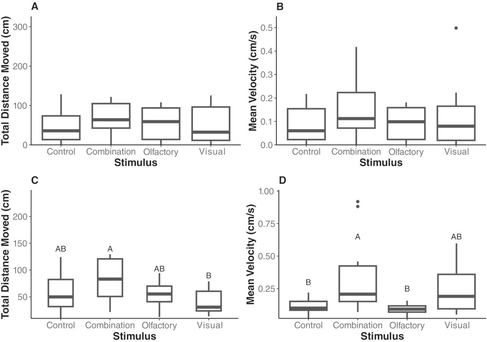
Distributions of distance moved and mean instantaneous velocity of R. dominica (A–B) and S. oryzae (C–D) exposed to headspace extracts of crickets and cricket visual cues.

Credits: Hetherington et al (2025)

2.1 Loading, wrangling, and plotting the data¶

We will focus on how these pests behave under different treatment conditions (Figure 3):

Visual: Pests are exposed to visual cues of crickets
Olfactory: Pests are exposed to chemical extract cues from crickets
Combined: Pests are exposed to both visual and olfactory cues
Control: Nothing special going on

Ultimately, we want to check whether visual or smell cues are enough to deter pest behavior, without having actual crickets around rice depots.

# Load ethology (animal behavior) data for both pest species and all four treatments

etho = pd.read_csv('Cricket_Ethovision.csv')
print(etho.shape)
etho.head()

(120, 19)

How does our data actually look like?

As usual, let’s do some jitterplots—which are more informative than boxplots
We also draw the 95% confidence intervals in black
And we also draw the standard deviation in red
Make sure to add grid lines so that we can check if the standard deviations are of similar size or if confidence intervals overlap

pests = ['LGB', 'RW']
effects = ['Total Distance', 'Velocity']
stimuli = ['Control', 'Combination', 'Olfactory', 'Visual']

fig, ax = plt.subplots(2,2, figsize=(9,5), sharex=True)
for i in range(len(pests)):
    ax[i,0].set_ylabel(pests[i], fontsize=fs)

    for j in range(len(effects)):
        ax[0,j].set_title(effects[j], fontsize=fs)
        ax[i,j].set_facecolor('snow')
        ax[i,j].set_xticks(range(len(stimuli)), stimuli, fontsize=fs)
        ax[i,j].grid(axis='y', zorder=1)

        df = etho.loc[etho['Species'] == pests[i] , ['Treatment', effects[j]] ]

        for k in range(len(stimuli)):
            yvals = df.loc[ df['Treatment'] == stimuli[k], effects[j] ]
            ci = stats.t.ppf(0.975, len(yvals)-1)*yvals.sem()
            std = yvals.std()/2

            ax[i,j].scatter(k + nudge[:len(yvals)], yvals, color=colors[k], marker=markers[k], ec='gray', lw=0.5, zorder=2, alpha=0.75)
            ax[i,j].errorbar(k , yvals.mean(), yerr=ci, color='k', mew=1.5, elinewidth=1.5, capsize=5, mfc='w', marker='D', zorder=3)
            ax[i,j].errorbar(k-0.2 , yvals.mean(), yerr=std, color='r', elinewidth=1.5, capsize=0, marker='', zorder=3)

fig.tight_layout();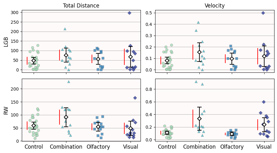

Is our data homoscedastic?

For LGB, the red lines look roughly the same size. You can imagine that these red lines would be more similar if we remove the obvious outliers.
For RW, the distance data looks homoscedastic—the “Combination” and “Visual” red lines will be shorter once we remove the single outlier.
- But the velocity data is not homoscedastic. Even without outliers, the “Combination” and “Visual” red lines aren’t as short as the “Control” and “Olfactory” ones.

(If your PI/Reviewer forces you to “verify” this assessment numerically, you can do a Levene’s test with stats.levene.)

Is our data normal-ish?

Let’s do Q-Q plots for both pests and both behaviors
We are going to keep all four conditions in the same plot:
Remember that for Q-Q plots, we mainly care if points follow the identity line (or any other line). Not so much the actual x- and y-axes values.
- To avoid points overlapping each other, we are going to horizontally offset each treatment
- This offset value is the mean behavior value (so it is large for distances but small for velocities)
- We do offset*k to move the offset with each behavior

quantiles = np.linspace(0.1, 0.9, 10)

fig, ax = plt.subplots(2,2, figsize=(7,4), sharex=False)
for i in range(len(pests)):
    ax[i,0].set_ylabel(pests[i], fontsize=fs)

    for j in range(len(effects)):
        ax[0,j].set_title(effects[j], fontsize=fs)
        ax[i,j].set_facecolor('snow')

        df = etho.loc[etho['Species'] == pests[i] , ['Treatment', effects[j]] ]

        # Each Q-Q line will have a horizontal offset equal to the mean effect value
        offset = df[effects[j]].mean()

        for k in range(len(stimuli)):
            yvals = df.loc[ df['Treatment'] == stimuli[k], effects[j] ]

            dataq = np.quantile(yvals, quantiles)
            normq = stats.norm.ppf(quantiles, yvals.mean(), yvals.std())

            # Notice how we add a horizontal offset to the Q-Q plots
            ax[i,j].scatter(offset*k + dataq, normq, color=colors[k], marker=markers[k], ec='gray', lw=0.5, zorder=2, alpha=0.75)
            ax[i,j].axline((offset*k + dataq[0], dataq[0]), slope=1, c=colors[k])

fig.tight_layout();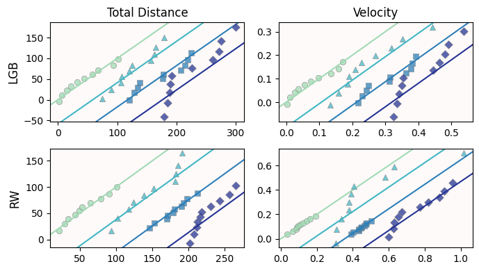

Is our data normal-ish?

For LGB, the ethology values seem normal-ish except for the “Visual” treatment (purple diamonds).
For RW, the ethology values seem normal-ish except for the “Combined” treatment (aqua triangles).

2.2 One-line loops and Multiple group testing¶

Let’s focus on the rice weevils (RW) for the rest of the assignment.

df = etho.loc[etho['Species'] == 'RW', ['Treatment'] + effects ]
df.head()

Since our data for “Total Distance” is mostly normal-ish (3 out of 4 samples) and homoscedastic, let’s do a Tukey’s HSD test.
The stats.tukey_hsd requires a list of samples; one item per sample

Python has a way to summarize simple loops in a single line for convenience. The loop in the cell below is equivalent to:

samples = []
for stim in stimuli:
    sample = df.loc[ df['Treatment'] == stim, 'Total Distance' ]
    samples.append(sample)

samples = [ df.loc[ df['Treatment'] == stim, 'Total Distance' ] for stim in stimuli]

We now use tukey_hsd: Notice the * at the beginning of our list samples.
We can then see the p-values as a 2D NumPy array with .pvalue (as with other tests)
For better visualization, we transform the 2D array into a DataFrame with appropriately named indices and columns.

# Tukey HSD test
hsd = stats.tukey_hsd(*samples)
pd.DataFrame(hsd.pvalue, stimuli, stimuli)

It seems that there are no differences between most of the treatments.
However, the difference between the “Combination” and “Visual” treatments is barely above 0.05.
This would suggest that it is worth exploring that difference further.
Looking back at the scatterplot, there is some overlap between their 95% confidence intervals, but not thaaat much, so a 0.05 p-value makes sense.
But more importantly, this overlap is small when compared to the rest of overlaps (Control vs Combination, Control vs Olfactory, etc.)

2.3 But what about just doing pairwise Welch’s instead?¶

For comparison, let’s consider all possible pairs (six in total), and do a Welch’s for each pair
The p-values are then adjusted for multiple tests (Benjamini-Hochberg)

pvalues = pd.Series()
for i in range(len(samples) - 1):
    for j in range(i+1, len(samples)):
        key = f'{stimuli[i]} vs {stimuli[j]}'
        pvalues.loc[key] = stats.ttest_ind(samples[i], samples[j], equal_var=False).pvalue

pvalues = pd.Series(stats.false_discovery_control(pvalues), index=pvalues.index)
pvalues

Control vs Combination      0.178206
Control vs Olfactory        0.695586
Control vs Visual           0.695586
Combination vs Olfactory    0.178206
Combination vs Visual       0.178206
Olfactory vs Visual         0.695586
dtype: float64

Notice that “Combination” vs “Visual” is now 0.18, well above the 0.05 threshold.
Even if you set equal_var = True (and do Student’s t-tests), the corrected p-value is 0.11, still much larger than 0.05.

3. Installing new packages¶

Switching gears: if you recall at the beginning of the course, you created a conda environment. This is the environment that you activate before doing anything. And when you created that environment at the beginning of the semester, you installed several packages alongside it (NumPy, SciPy, pandas, etc.)

But what if you need an extra package? Like SciKit Post Hoc to get access to many more powerful statistical tests not yet implemented in SciPy?

You can of course install it!

Make a note of this cell and close the Notebook and anaconda. For example, you can copy/paste it in a text editor/google docs/etc.
Open your conda prompt/terminal (depending on whether you’re using Windows or Mac) as usual, alongside the typical

(base) something.something$ conda activate myenv [<or however you named your environment>]

Make sure your terminal/prompt says myenv (or however you named your environment) at the begining:

(myenv) something.something.$

Then go to anaconda module repository and search for scikit-posthocs
Click on the most downloaded/used option
Check the installation instruction command
Copy/paste the command in your conda prompt/terminal
And that’s it! You’ve just installed a new package in your environment and you can keep doing more stats!
Keep reading the final part of the assignment to make sure the installation was sucessful. Remember to re-lauch the Notebook

(myenv) something.something.$ jupyter notebook

Important: If you have issues, we can troubleshoot at the beginning of the next class.¶

4. Checking `scikit_posthocs` and rice weevils velocity¶

To make sure your installation was successful, you should be able to import your new module:

# Test your newly installed module
import scikit_posthocs as posthocs

Make sure you run all the prior cells.

And now we can check the differences in weevil velocity depending on the pest treatment.

Since velocity data is not homoscedastic, we cannot do Tukey’s HSD
The Q-Q plot for the “Combined” treatment was wildly not normal, so we better use a non-parametric test.

In the non-parametric case, we have to start with an omnibus test: Kruskal-Wallis. Just like with Tukey HSD, we need a list with samples. Notice the * in front of samples.

samples = [ df.loc[ df['Treatment'] == stim, 'Velocity' ] for stim in stimuli]

stats.kruskal(*samples, nan_policy='omit') #ignore NaNs if any

KruskalResult(statistic=16.674726775956287, pvalue=0.0008243751909988866)

We have a tiny p-value of 0.0008, which suggests that treatment might explain some of velocity variance among weevils.
We switch to a Conover post-hoc test to tease apart individual differences.
Notice that we do not use a * in this case.

conover = posthocs.posthoc_conover(samples, p_adjust='fdr_bh')
conover

That’s not that readable: add column and index names

conover.columns = stimuli
conover.index = stimuli
conover

The cool thing of the posthocs module is that you can also use DataFrames as inputs
We specify the column name with the values we care (Velocity)
And the column name that distiguishes which treatment is which (Treatment)

posthocs.posthoc_conover(df, val_col='Velocity', group_col='Treatment', sort=True, p_adjust='fdr_bh')

In this case, we see that Control and Olfactory are similar (0.38) and form one group.
Combination and Visual are also similar (0.30) and form another group.
These two groups are different from each other.
These results match perfectly our jitterplots and the overlaps—or lack thereof—of their confidence intervals.

Congratulations, you’re done!¶

Submit this assignment by uploading it to the course Canvas web page. Go to the “Pre-class assignments” folder, find the appropriate submission folder link, and upload it there.

See you in class!

References¶

Hetherington, M. C., Sakka, M. K., Abshire, J., Maille, J. M., Stoll, I., Athanassiou, C. G., Scully, E. D., Gerken, A. R., & Morrison, W. R. (2025). Nonconsumptive effects of parasitoids and predators in stored products: the impact of <scp> Theocolax elegans </scp> and other field‐collected predators on the foraging of lesser grain borer and rice weevil. Pest Management Science, 81(11), 7529–7541. 10.1002/ps.70230

✅ Put your name here¶