Day 25: In-Class Assignment

✅ Put your name here
¶

✅ Put your group member names here
¶

How heavy was a diplodocus?¶

Complete fossil skeleton of a diplodocus dinosaur.

Learning goals of today’s assignment¶

Compute and plot confidence bands for allometry models
Use the linear model to estimate the weight of the diplodocus and estimate its confidence interval

Assignment instructions¶

Work with your group to complete this assignment. Instructions for submitting this assignment are at the end of the Notebook. The assignment is due at the end of class.

Importing the modules that we will need¶

Before we start anything, it is good practice to have all our imports as the first Python cell

import numpy as np
import matplotlib.pyplot as plt
import pandas as pd
from scipy import stats
from sklearn import metrics

1. Allometry, revisited¶

In this Notebook we will recall the femur-humerus-weight allometry dataset from Days 09 and 10. In those assignments, we set to model body weight based solely on humerus and femur’s circumferences based on an allometric relationship:

$\log_{10}(\text{Body Mass}) = b\times\log_{10}(\text{femur + humerus circumference}) + \log_{10}(a),$
(1)
¶

for some constant values $a, b$ .

Raw OLS regression for body mass estimation and percent prediction error of body mass proxies

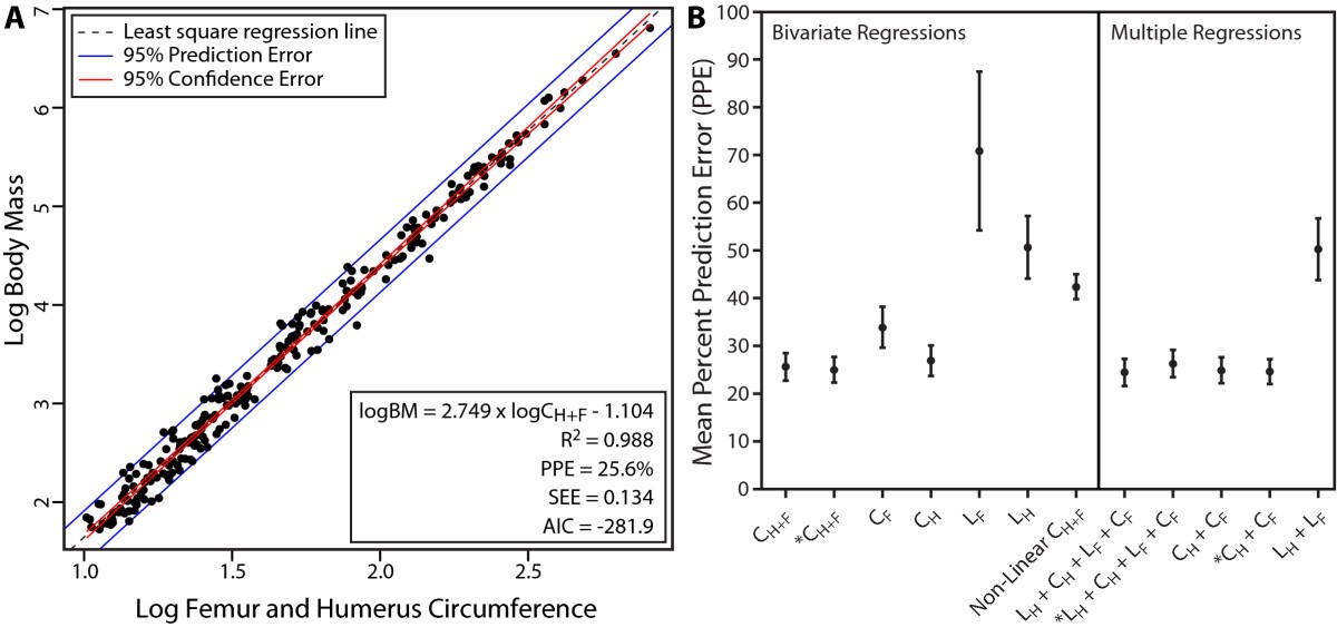
Credits: Campione and Evans (2012)

We will use data from Campione and Evans (2012) to compute a linear model to then predict the weight of various dinosaurs using their fossil data.

1.1 Data loading and visualization¶

✅ Task 1

Load the '12915_2012_575_MOESM1_ESM.XLS' file (attached in Canvas). Mind the casing. Notice that it is an Excel file with various Sheets.
Check how to use the sheet_name parameter so that you have two DataFrames: one for existing quadrupeds and another for dinosaurs’ measurements.
Check the index_col parameter to have the species names as indices instead of 0,1,2,...
You should have 255 and 8 data points for existing animals and dinosaurs, respectively.

# Load with pandas

✅ Task 2

Compute a linear model between log₁₀ body mass and log₁₀(femur + humerus circumferences), like the allometric relationship indicates above (in the past classes, we only used femur data).
Obviously, we can only use existing animals’ data because we have no bodymass data for dinosaurs.
Make sure you are using log₁₀ (log base 10), not natural log.
- The actual base does not matter, but we want to stay consistent with the source paper.
Compute the $R^2$ determination coefficient of this model.
Do the model and $R^2$ values match those displayed by Campione and Evans (2012) in Figure 4 (the figure displayed above)?

Hint: It will be easier later if you define variables true_x and true_y from the get-go

# Your linear model
# Print the intercept, slope, and R2

✅ Task 3

Make a scatterplot of the data
Draw the best-fit line
Make sure your axes are labeled

# Your plot

✅ Question 4

From both the statistics and the visualization, do you think femur+humerus circumferences are good proxies of body weight?
What does $R^2$ mean in femur-humerus-bodymass terms?

✎ Put your answer here.

✅ Question 5

From both the statistics and the visualization, do you expect the 95% confidence band to be wide or tight around the best-fit line?

✎ Put your answer here.

2. Confidence and prediction bands¶

You will review the code to compute confidence bands for linear models. You essentially just need to copy/paste the code from the pre-class and make the relevant edits.

✅ Task 6

Compute and print the mean square error:
$\text{MSE} = \frac1{n-2}{\sum_{i=1}^n{{(y_i-\hat{y_i})^2}}}.$
(2)
Compute the sum of squared x-axis deviations:
$SS_x = \sum_{i=1}^n(x_i - \bar{x})^2.$
(3)

# Your code

✅ Task 7

Define a sequence of 100 x-axis values, going from the minimum to the maximum observed.
For each x value of this sequence, compute its standard error of the linear prediction:
$s_{\hat{y}} = \sqrt{\text{MSE}\times\left(\frac1n + \frac{(x-\bar{x})^2}{SS_x}\right)}.$
(4)
For each x value, also compute its prediction error:
$\text{pred}_{\hat{y}} = \sqrt{\text{MSE}\times\left(1 + \frac1n + \frac{(x-\bar{x})^2}{SS_x}\right)}.$
(5)

# Your code

✅ Task 8

Finally, copy/paste your scatterplot from T3
Add code lines so it also displays the 95% confidence band
Add the 95% prediction band

Note: The confidence band is quite tight and the best-fit line might overshadow it. You might need to draw a very thin best-fit line (lw = 0.1) to actually see this band.

# Your code

✅ Question 9

Remember that the ultimate goal is to predict the weight of a dinosaur. Having a good estimate of its weight is crucial to understand how it moved and behaved, how it ate, and in general, how it formed part of the whole prehistoric ecology.

Imagine that you are a PhD student in the Dinosaur Lab. Would you use confidence or prediction intervals to estimate the dinosaur’s weight? You’ll base your next 4 years of research based on this estimation.

✎ Justify your answer.

3. Predicting dinosaur weights¶

✅ Task 10

Use your allometric model to predict the bodymass for the eight dinosaur fossil records.
Remember that you’ll be predicting log₁₀ gram values: you’ll need to power them and divide by 1000 (so you have kilograms).
Use the .astype function with dtype = int to force the display of values to be integers for better readability.

Hint You should get values in the same ballpark as those in Table 6 (last column) from Campione and Evans (2012).

# Your code

✅ Task 11

Make two Series: for the lower and higher ends of the 95% confidence interval of these bodyweight predictions, respectively.
Make sure your results are displayed in kilograms

# Your code

✅ Task 12

Same as Task 12, except you’ll be looking at 95% prediction intervals.

Note: The Table 6 does not do prediction intervals. It does something else based on the mean percent prediction error (PPE), which is related to MSE. Don’t worry about it.

# your code

✅ Task 13

Use pd.concat to concatenate the five Series you made in T10, T11, and T12 into a single DataFrame.
Change the column names so they are more descriptive.

# Your tests

✅ Question 14

Now that you have a better sense of how the confidence and prediction intervals compare to each other, would you change your answer for Q9 or would you double down?

✎ Put your answer here

✅ Task 15: A side note on science communication

If you tell me that on average a diplodocus weighted 10635kgs or 23400lbs, I might only register that it was very heavy. People in general have a hard time conceptualizing really large or really small numbers. Which is why it is often useful to associate those big numbers to something more relatable.

For example, an average 2025 Ford F-150 weights about 5,175 lbs or 2350 kgs.

How many F-150s is an average diplodocus worth?
What is the maximum possible weight (with 95% of confidence) for a triceratops (in F-150 terms)?
What other relatable weight “units” can you think of?

# Your code here

Congratulations, you’re done!¶

Submit this assignment by uploading it to the course Canvas web page. Go to the “In-class assignments” folder, find the appropriate submission link, and upload it there.

See you next class!

References¶

Campione, N. E., & Evans, D. C. (2012). A universal scaling relationship between body mass and proximal limb bone dimensions in quadrupedal terrestrial tetrapods. BMC Biology, 10(1). 10.1186/1741-7007-10-60

✅ Put your name here¶

✅ Put your group member names here¶