Day 26: In-Class Assignment

✅ Put your name here
¶

✅ Put your group member names here
¶

Predicting avian growth with sigmoid functions¶

View of a nesting site with several imperial shags Phalacrocorax atriceps.

Learning goals of today’s assignment¶

Use curve_fit to fit non-linear models to determine avian growth based on days since hatching

Assignment instructions¶

Work with your group to complete this assignment. Instructions for submitting this assignment are at the end of the Notebook. The assignment is due at the end of class.

Importing the modules that we will need¶

Before we start anything, it is good practice to have all our imports as the first Python cell

import numpy as np
import matplotlib.pyplot as plt
import pandas as pd
from scipy import stats, optimize
from sklearn import metrics

Background¶

This paper evaluates the effectiveness of various sigmoid-like growth models in analyzing postnatal growth in the imperial shag (Phalacrocorax atriceps). The study finds that the Richards model provides the most accurate estimates of adult size and growth parameters, outperforming traditional three-parameter models, which can introduce bias. Overall, the combination of the Richards equation and nonlinear mixed models offers a robust approach for studying avian growth.

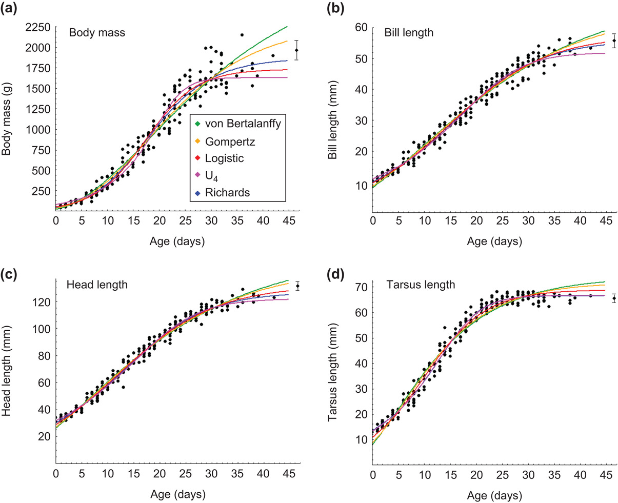
Growth curves of female chicks of the imperial shag (n = 33) for (a) body mass, (b) bill length, (c) head length and (d) tarsus length. Curves were obtained from nonlinear mixed models applied to von Bertalanffy (green), Gompertz (orange), logistic (red), U4 (pink) and Richards (blue) models. Measured values are shown as circles. Mean ± SD of adult values are shown.

Credits: Svagelj et al (2019)

The data comes from:

Svagelj, W.S., Laich, A.G. and Quintana, F. (2019) Richards’s equation and nonlinear mixed models applied to avian growth: why use them?. Journal of Avian Biology, 50

✅ Question 1

The five models studied by Svagelj et al (2019) are sigmoid functions. A sigmoid curve looks like a stretched-out S. Unlike linear or power functions, sigmoid curves do not grow indefinitely but have a defined limit (asymptote).

Do you think sigmoid functions are a reasonable choice to model growth?

✎ Put your answer here.

2. Keeping track of imperial shag (cormorant) growth¶

✅ Task 2

Load the 'RGM_data.xlsx' file (attached in Canvas).
You should have 209 rows.
- ID: Identification tag of the individual bird measured
- t: Days since birth
- The rest of the columns are length and mass measurements of the bird

# Load with pandas

✅ Question 3

As a rule of thumb, whenever you are doing regression, you want your measurements to be independent—the value from one row has no influence whatsoever on any other row?

Do you think the measurements in our dataset are 100% independent?

Note: Whenever you have data with some dependence, you can use a Mixed-effect model to take into account such dependencies. Mixed models go beyond the scope of this course and we will ignore them for the rest of the assignment.

✎ Put your answer here.

3. Fitting a logistic model to bill lengths¶

The “simplest” sigmoid model Svagelj et al (2019) try is a logistic one. Based on the bird’s age $t$ , its bill length is modeled according to the function:

L(t) = \frac A{1 + \exp(k\times(t-T))}.

(1)

The $A$ parameter is the asympotic value: the function will never go beyond this value. $k,T$ are shape and shift parameters.

✅ Question 4

How many parameters does the logistic model fit?
Which one is the independent (x-axis) variable?

✎ Put your answer here.

✅ Task 5

Define a logistic function as described above. Remember that the independent variable must go first.

# your logistic model

✅ Task 6

Use curve_fit to figure out which are the optimal parameters to estimate bill length.

Note: You might get a RuntimeWarning. This is not an error but a word of caution that Python is unsure of some of the math. In practical terms, it means: visualize your results and double check they look ok (which is something you should always do, anyway.)

# Your code

✅ Task 7

Use your logistic model to predict bill lengths based on the actual ages we have in the data.
Compute the $R^2$ coefficient by comparing the real bill lengths in the data against the predicted lengths.

# R2

✅ Question 8

Just by looking at the numbers, do you think the logistic model is a good model for bill length?

✎ Put your answer here.

✅ Task 9

Now define an array of x-axis values that go from 0 to 60—we choose 60 because the oldest bird was 50.
Predict a corresponding array of y-axis values based on your logistic model

# your code

✅ Task 10

Make a scatterplot with the actual age and bill length values from the data
Use the arrays from T9 to draw the best-fit logistic curve
Does it match your intuition from Q8? Do the extrapolated values look reasonable?

# your plot

✅ Question 11

Without doing any extra coding:

Do you think a sigmoidal curve—like the logistic one—is more realistic in this case compared to a linear or polynomial curve?

✎ Put your answer here.

4. Fitting a Gompertz model—giving `curve_fit` a hand¶

The logistic model looks very reasonable already. But it is not the only sigmoid curve out there. The Gompertz model is another sigmoid curve fairly common when modeling growth:

L(t) = Ae^{-e^{-k(t-T)}} = A\times\exp(-\exp(-k\times(t-T))).

(2)

Like the logistic case, $A$ determines the maximum of the model (asymptote) and $k,T$ determine shift and shape.

✅ Task 12

Define a gompertz function as described above. Keep track of your parentheses!
Use curve_fit to find the optimal parameters

# Your code

✅ Task 13

Copy/paste and edit your prediction code from T9 and your plot code from T10
Does the Gompertz curve look reasonable? (We’ll fix it in the next Task).

# Copy/past T9 and T10

4.1 The importance of an initial guess¶

The parameters we got make no sense. We need to give curve_fit some help!

Every optimization algorithm has the following steps:

Start with a guess of the optimal parameters.
Check how good of guess step 1 was (check the least squares function).
Update the guess so the least squares function improves.
Repeat steps 1–3 until you reach the solution.

However, if your initial guess is far away from the actual solution, it is possible that the algorithm will be unable to reach any meaningful answers. The initial guess maters: the closer to the actual solution, the better!

Notice that curve_fit has a p0 argument where you can give an initial guess. What happens by default if you don’t provide one?

✅ Task 14

Copy/paste again your prediction code from T9, except that your Gompertz model will use the parameters from guess instead of those from curve_fit you used before
Copy/paste the scatter and line plot code to check how good this guess is
Wiggle the guess values so that the curve looks closer to the actual values. What if you increase or reduce their values (keep them positive though)? Do not spend more than 5 minutes in this Task.

Remember: you want a good guess, not to solve the actual optimization problem (that’s what curve_fit is for)

We start with A = 60 because that seems to be the max bill length.

# Improve the guess

guess = [60, 0.5, 6]

✅ Task 15

Repeat T12 , but now curve_fit has the p0 = guess argument
Copy/paste your code from T13. Does the curve look reasonable now?

5. Which is the better model?¶

There are several computational and statistical ways to determine which model is the “better” one, like comparing their mean square errors (MSE), $R^2$ coefficients, conditional numbers of the covariance matrix of the parameters, or their Akaike Information Criterion (AIC).

However, these approaches are agnostic: they do not take into account actual domain knowledge. Domain knowledge should always guide your data science.

Consider the following. Svagelj and Quintana (2007) measured the length of imperial cormorants in two years. The summary is:

Bill length (mm)	Males	Females
2004	58.7 ± 2.2	55.3 ± 2.3
2005	58.9 ± 2.2	56.2 ± 2.2

The A parameter of either the logistic or Gompertz models indicate the asymptote: the maximum possible value attained by the model.

✅ Task 16

With all of the above in mind, if you were part of the Cormorant Lab, which model would you prefer to model bill lengths? Explain your answer.

# Your code

✎ Put your answer here.

Congratulations, you’re done!¶

Submit this assignment by uploading it to the course Canvas web page. Go to the “In-class assignments” folder, find the appropriate submission link, and upload it there.

See you next class!

References¶

Svagelj, W. S., Laich, A. G., & Quintana, F. (2019). Richards’s equation and nonlinear mixed models applied to avian growth: why use them? Journal of Avian Biology, 50(1). 10.1111/jav.01864
Svagelj, W. S., Laich, A. G., & Quintana, F. (2019). Richards’s equation and nonlinear mixed models applied to avian growth: why use them? Journal of Avian Biology, 50(1). 10.1111/jav.01864
Portet, S. (2020). A primer on model selection using the Akaike Information Criterion. Infectious Disease Modelling, 5, 111–128. 10.1016/j.idm.2019.12.010

✅ Put your name here¶

✅ Put your group member names here¶

Predicting avian growth with sigmoid functions¶

Learning goals of today’s assignment¶

Assignment instructions¶

Importing the modules that we will need¶

Background¶

2. Keeping track of imperial shag (cormorant) growth¶

3. Fitting a logistic model to bill lengths¶

4. Fitting a Gompertz model—giving curve_fit a hand¶

4.1 The importance of an initial guess¶

5. Which is the better model?¶

Congratulations, you’re done!¶

✅ Put your name here
¶

✅ Put your group member names here
¶

4. Fitting a Gompertz model—giving `curve_fit` a hand¶