Day 10 Pre-Class Assignment

✅ Put your name here
¶

Python Modules: Fleshing out NumPy¶

Learning goals for today’s assignment¶

Import NumPy into Python and create an manipulate NumPy arrays.
Use NumPy to do simple calculations with arrays

Assignment instructions¶

Watch the videos below, do the readings linked to below the videos, and complete the assigned programming problems. Please get started early, and come to office hours if you have any questions! Make use of Slack as well!

This assignment is due by 11:59 p.m. the day before class, and should be uploaded into appropriate the “Pre-class assignments” submission folder. Submission instructions can be found at the end of the notebook.

A brief aside on Jupyter notebooks¶

Before you get started with this notebook, take a few minutes to make sure you are feeling comfortable with Jupyter notebooks at this point in the course.

If you still have any questions about how they work, or how to better use them, post your thoughts on our Slack channel.
It is really important to keep in mind that Jupyter notebooks are based on cells. This is a markdown cell, for example. Because you can execute the cells in any order you wish, it is up to you to keep track of what has been done, or not. If it helps, you can make an initial habit of running all cells from the top down, although there will be cases where you won’t want to do that.
It is worth taking a few minutes to get better at keyboard shortcuts, which will make using the notebooks much more efficient; and, learning some markdown is also helpful. Both are in this webpage, and you can also do a web search to find other tutorials on these topics.
One of the best things about the notebooks is rapid prototyping of code. This means: try something quickly, delete it and move on. With the keyboard shortcuts, this becomes quite fast. Suppose you want to know what 4 + 5 * 3 will give. The steps are simple:
- press Esc to get out of the cell you are in (go into command mode)
- press B to create a cell below (or A for above - your choice)
- press Return/Enter to enter/activate the cell (to go into edit mode)
- type in your test (e.g., 4 + 5 * 3)
- press shift + Enter
- press Esc to get out of the interior of the cell (go from edit to command mode)
- press X (or D twice) to delete that temporary cell
Sometimes, when trying to debug your code, it can be really useful to be able to see the line numbers (usually Python will tell you in which line it found an error). To do this:
- press Esc to get out of the cell you are in (to go into command mode)
- press Shift + L to turn on lines numbers

This may seem like a lot of steps, but once you memorize the shortcuts, you can rapidly create, use and delete cells. And using line numbers is a good way to better review your code and discuss it with someone else. When you have an error, this is best way to quickly isolate parts of the code to test them.

Try it now!

Part 1. Getting familiar with NumPy¶

Okay, now let’s get to the subject of this pre-class assignment: NumPy.

As you learned in the previous course material, Python comes with a large number of extremely useful libraries. In fact, Python itself is a rather small language on its own; it’s true power is the myriad of libraries developed for it. In our realm of computational modeling, a core library is NumPy, which translates to “Numerical Python”. NumPy allows you to do mathematical operations both more easily (from a coding perspective) and faster (in the sense of how long you need to wait for the result).

As with other libraries, you include NumPy through an import command. Execute the next cell.

import numpy as np

Note that NumPy gets imported, but also gets renamed as “np”. You don’t need to use “np” if you don’t want to; but, in the Python community, everyone else does and it makes it easier for people to read each other’s code if we all use the same conventions. NumPy is vast. We will be learning aspects of NumPy throughout the entire semester, and this assignment is just the beginning of that journey.

Why do we have the dot notation in which we will make calls to libraries with np.?

The reason is that Python is huge and some of the libraries have overlapping functionalities. For example, you may find that NumPy contains libraries that also exist in other modules you learn later in the semester. By using the dot notation, you can be sure you are using the library of your choice, and you are free to switch between them throughout your code. Sometimes you will use dots twice, as in np.random.default_rng(42).

For now, we will focus on the key element of NumPy: the array.

✅ Task 1:

Now, watch the following video to learn about the basics of NumPy arrays and how they differ from lists, which have been your main tool for storing information up to this point.

from IPython.display import YouTubeVideo
YouTubeVideo("g7epZeDA_lQ",width=640,height=360)

✅ Task 1 (continued)

Explain, in your own words, some of the similarities and differences between standard Python lists and the NumPy arrays.

✎ Put your answer here!

Manipulating NumPy arrays and performing mathematical operations¶

Now that you understand a bit more about the NumPy array object in Python, watch the following video to understand how we can manipulate NumPy arrays and use them to perform mathematical operations, which is precisely what NumPy arrays were built for!

YouTubeVideo("V2C9expTF1o",width=640,height=360)

✅ Question 2

If you had two arrays of the same length and wanted to create a new array that is the product of the first two, how would you do that?

✎ Put your answer here

✅ Question 3

What functions can I use to find the sum, minimum value, maximum value, and average value of a NumPy array? How do I call these functions? (Provide some example code in your response).

✎ Put your answer here

Part 2. Working with NumPy Arrays¶

As you’ve learned at this point, at the core of NumPy is a data type called an array. An array is like a Python list, but has some very different features. It is best to not confuse them, even if sometimes they might be interchangable. All other opertions in NumPy, and many other Python libraries used for computations, will assume you are using this array type.

The first thing you need to learn to do is create an array, and there are several ways of doing this depending on your goals. Let’s learn two related methods now.

2.1 `np.arange`¶

You already found this function in the last In-Class, but we did not discuss much about it then. The np.arange function is similar to the range function: it creates an array where the entries go from a minimum to a maximum value using an even step size. The arguments are:

The minimum value
The maximum value
The step size

so the following command:

np.arange(0,100,5)

array([ 0,  5, 10, 15, 20, 25, 30, 35, 40, 45, 50, 55, 60, 65, 70, 75, 80,
       85, 90, 95])

creates an array that goes from 0 to 100 in steps of 5.

Note: much like the range command, it does not include the maximum value as an entry in the array.

2.2 `np.linspace`¶

The np.linspace function is similar, in that it creates an array where the entries are linearly spaced. But it has one important difference. Its three arguments are:

The minimum value
The maximum value
The number of elements

so the following command:

np.linspace(0.1,1,10)

array([0.1, 0.2, 0.3, 0.4, 0.5, 0.6, 0.7, 0.8, 0.9, 1. ])

creates an array with 10 elements, linearly (or evenly) spaced, from 0.1 to 1.0.

Unlike the range function, this is inclusive of the endpoints by default.
In other words, it includes entries for both the minimum and maximum values.
Note 1: this is good for dealing with floats!
Note 2: You can exclude the endpoint (like the np.arange case) with the argument endpoint=False.

Now, say, to create a set of $x$ values spanning $[0,2 \pi]$ , you can use np.linspace instead of a while loop!

There is a lot of documentation on the web, such as this. These “doc pages” can also be accessed directly in Jupyter using “?”:

np.linspace?

Since these functions are so similar, it is important not to get them mixed up! Look at the example code below and answer the questions about the differences between np.arange and np.linspace:

# comparing arange to linspace
my_array_range = np.arange(0,10,1) # Make sure you understand how this line is different...
my_array_linspace = np.linspace(0,9,10) # ... than this line
print("Using arange I get:", my_array_range)
print("Using linspace I get:", my_array_linspace)

Using arange I get: [0 1 2 3 4 5 6 7 8 9]
Using linspace I get: [0. 1. 2. 3. 4. 5. 6. 7. 8. 9.]

✅ Question 4

Now, in your own words, describe what these functions do.
When do you think you would chose to use one over the other?

✎ Put your answer here.

2.3 `np.zeros` and `np.ones`¶

Believe it or not, a common way to initialize NumPy arrays is by filling them with zeros. For this you can use the np.zeros function:

np.zeros(10)

array([0., 0., 0., 0., 0., 0., 0., 0., 0., 0.])

which gives us an array of 10 elements, each one equal to zero. Similarly, we could use the np.ones function:

np.ones(10)

array([1., 1., 1., 1., 1., 1., 1., 1., 1., 1.])

to give us an array full of ones.

Notice that these zeros and ones are floats: they are printed as 0. and 1. instead of 0 and 1, respectively (look at the dot).
You can make the zeros and ones ints or bools by adding the argument dtype = int or dtype = bool, respectively.

2.4 No mixed data types!¶

The arrays look a lot like lists. But, a key difference is that you cannot have mixed types inside of the array. For example, try this code:

my_list = [1, 3.1415, 'PLNT_SCI'] # this list has three different types in it: integer, float and string
conv_to_array = np.array(my_list) # this converts a list to an array
print(conv_to_array)

['1' '3.1415' 'PLNT_SCI']

✅ Question 5

What are the types of the elements in the new array?
Are they the same as the original list?
Are they all the same as each other?

Try modifying the list with different initial variables types to see if you can figure out the rule Python uses for setting the element type in the array when the conversion step happens.

# code to examine different types of lists to see what np.array does to them

2.5 Mathematical operations¶

One of the greatest parts of NumPy arrays is that you can change all elements using a single line of code!

This greatly simplifies a lot of the work we’ve been doing with lists and loops.

Let’s try some mathematical operations on arrays.

✅ Task 6

Make an array that contains the numbers 0 through 9.
Multiply all the elements by 3, then subtract 7.

# Put your code here.`

✅ Task 7

Make an array of the first 100 positive integers and save it as first_100.
Compute and print the square of the array as print(first_100**2).

# Put your code here

2.6 NumPy functions¶

NumPy also contains its own math libraries, highly tuned to be used with NumPy arrays. As always, to access those you need to use the “dot notation”. For example, run this cell:

# This code cell uses four NumPy methods:
# linspace, pi, sin and cos
x_values = np.linspace(0, 2*np.pi, 200)
sin_times_10sin = np.sin(x_values) * np.sin(10*x_values)
print( sin_times_10sin )

[ 0.00000000e+00  9.80260394e-03  3.72535696e-02  7.67791032e-02
  1.20038202e-01  1.57209145e-01  1.78535813e-01  1.75919224e-01
  1.44330022e-01  8.28375267e-02 -4.90191280e-03 -1.10785831e-01
 -2.23042716e-01 -3.27567726e-01 -4.09663151e-01 -4.55971284e-01
 -4.56354635e-01 -4.05476075e-01 -3.03860594e-01 -1.58277820e-01
  1.86360732e-02  2.09506448e-01  3.93994102e-01  5.51027293e-01
  6.61241132e-01  7.09339208e-01  6.86091488e-01  5.89716171e-01
  4.26458053e-01  2.10265007e-01 -3.84326464e-02 -2.94729806e-01
 -5.31836204e-01 -7.23969553e-01 -8.49231293e-01 -8.92137804e-01
 -8.45511544e-01 -7.11502903e-01 -5.01607526e-01 -2.35655052e-01
  6.01389667e-02  3.55859000e-01  6.21028266e-01  8.27860200e-01
  9.54265514e-01  9.86280695e-01  9.19644742e-01  7.60343124e-01
  5.24051174e-01  2.34530730e-01 -7.88500889e-02 -3.84206409e-01
 -6.50500007e-01 -8.50810563e-01 -9.65159020e-01 -9.82577298e-01
 -9.02202543e-01 -7.33282545e-01 -4.94099485e-01 -2.09938304e-01
  8.96698714e-02  3.74121133e-01  6.14978398e-01  7.88923642e-01
  8.80105785e-01  8.81638884e-01  7.96103385e-01  6.35016315e-01
  4.17351465e-01  1.67294675e-01 -8.84994436e-02 -3.23833341e-01
 -5.15746179e-01 -6.46843318e-01 -7.06930549e-01 -6.93793442e-01
 -6.13063871e-01 -4.77221586e-01 -3.03876180e-01 -1.13552897e-01
  7.27443940e-02  2.35903140e-01  3.60733066e-01  4.37435768e-01
  4.62365078e-01  4.38020259e-01  3.72308309e-01  2.77198707e-01
  1.66963406e-01  5.62387648e-02 -4.18403758e-02 -1.17202202e-01
 -1.63909092e-01 -1.80621084e-01 -1.70416002e-01 -1.40014971e-01
 -9.85384602e-02 -5.59767929e-02 -2.15930979e-02 -2.48181893e-03
 -2.48181893e-03 -2.15930979e-02 -5.59767929e-02 -9.85384602e-02
 -1.40014971e-01 -1.70416002e-01 -1.80621084e-01 -1.63909092e-01
 -1.17202202e-01 -4.18403758e-02  5.62387648e-02  1.66963406e-01
  2.77198707e-01  3.72308309e-01  4.38020259e-01  4.62365078e-01
  4.37435768e-01  3.60733066e-01  2.35903140e-01  7.27443940e-02
 -1.13552897e-01 -3.03876180e-01 -4.77221586e-01 -6.13063871e-01
 -6.93793442e-01 -7.06930549e-01 -6.46843318e-01 -5.15746179e-01
 -3.23833341e-01 -8.84994436e-02  1.67294675e-01  4.17351465e-01
  6.35016315e-01  7.96103385e-01  8.81638884e-01  8.80105785e-01
  7.88923642e-01  6.14978398e-01  3.74121133e-01  8.96698714e-02
 -2.09938304e-01 -4.94099485e-01 -7.33282545e-01 -9.02202543e-01
 -9.82577298e-01 -9.65159020e-01 -8.50810563e-01 -6.50500007e-01
 -3.84206409e-01 -7.88500889e-02  2.34530730e-01  5.24051174e-01
  7.60343124e-01  9.19644742e-01  9.86280695e-01  9.54265514e-01
  8.27860200e-01  6.21028266e-01  3.55859000e-01  6.01389667e-02
 -2.35655052e-01 -5.01607526e-01 -7.11502903e-01 -8.45511544e-01
 -8.92137804e-01 -8.49231293e-01 -7.23969553e-01 -5.31836204e-01
 -2.94729806e-01 -3.84326464e-02  2.10265007e-01  4.26458053e-01
  5.89716171e-01  6.86091488e-01  7.09339208e-01  6.61241132e-01
  5.51027293e-01  3.93994102e-01  2.09506448e-01  1.86360732e-02
 -1.58277820e-01 -3.03860594e-01 -4.05476075e-01 -4.56354635e-01
 -4.55971284e-01 -4.09663151e-01 -3.27567726e-01 -2.23042716e-01
 -1.10785831e-01 -4.90191280e-03  8.28375267e-02  1.44330022e-01
  1.75919224e-01  1.78535813e-01  1.57209145e-01  1.20038202e-01
  7.67791032e-02  3.72535696e-02  9.80260394e-03  5.99903913e-31]

✅ Question 8

Describe what you see

✎ Put your answer here.

We recently learned another library: matplotlib. Let’s combine them. The first thing you need to do is import that library:

import matplotlib.pyplot as plt

✅ Task 9

Plot the sin_times_10sin array versus your original x_values array.

Don’t worry, matplotlib’s ax.plot function can accept NumPy arrays as arguments!

Check the Axes detour from In-Class 09 if you need to check again how to use the Axes interface.

# plot of my function. You have the first line already
# (be sure to include axis labels!)

fig, ax = plt.subplots(figsize=(5,3))

2.7 Some numpy statistics operations¶

Finally, let’s learn just a few of the easy operations in NumPy for doing statistics. The cell below shows how easy it is to compute the sum, mean, median and standard deviation of a dataset:

ages_dataset = np.array([1,1,2,3,3,5,7,8,9,10,10,11,11,13,13,15,16,17,18,18,
18,19,20,21,21,23,24,24,25,25,25,25,26,26,26,27,27,27,27,27,
29,30,30,31,33,34,34,34,35,36,36,37,37,38,38,39,40,41,41,42,
43,44,45,45,46,47,48,48,49,50,51,52,53,54,55,55,56,57,58,60,
61,63,64,65,66,68,70,71,72,74,75,77,81,83,84,87,89,90,90,91])

print("The sum of the dataset is",np.sum(ages_dataset))
print("The mean of the dataset is",np.mean(ages_dataset))
print("The median of the dataset is",np.median(ages_dataset))
print("The standard deviation of the dataset is",np.std(ages_dataset))

The sum of the dataset is 3926
The mean of the dataset is 39.26
The median of the dataset is 36.0
The standard deviation of the dataset is 23.60026271040219

One useful way to visualize a dataset is with a histogram.

A histogram is constructed by “binning” data. For example, the data above could be binned into a number of age intervals (0-5, 5-10, 10-15, etc.). The x-axis of a histogram are the bins chosen for the data set, and the y-axis is the number of observations that fall into each bin. In Python, we can use the ax.hist() function from matplotlib to make one-dimensional histograms:

# a histogram of the ages with the data binned into increments of 10
fig, ax = plt.subplots(figsize=(5,3))
ax.hist(ages_dataset,bins=10)
ax.set_xlabel('Age')
ax.set_ylabel('Frequency');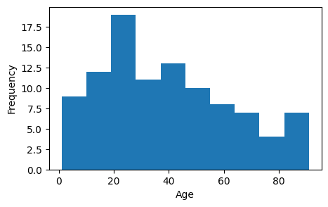

✅ Task 10

Try changing the bin size in the example below and note what happens to the data.

# Put your commented code here:

3. Reading in Data: Quadrupeds size measurements¶

We’ll be using Numpy to read in data from files in class, so let’s get some practice with that now. Along with this pre-class assignment, you should have also downloaded a file called quadrupeds_sample.csv. Make sure the file is in the same directory as this Notebook.

As with the saguaro data from prior assignments, we are using data from real research. The CSV file is a sample from Campione and Evans (2012). This is a research paper on allometry, continuing our work from the previous In-Class.

Campione, N.E., Evans, D.C. (2012) A universal scaling relationship between body mass and proximal limb bone dimensions in quadrupedal terrestrial tetrapods. BMC Biol 10(60).

3.1 Examining the Data¶

Take a moment to look at the contents of this file (quadrupeds_sample.csv) with an editor on your computer.

✅ Question 10

Describe the contents of the CSV.

What does the data look like?
- how many columns of data are there?
- what do the different columns of data represent?
- what kind of values/datatypes are in each column?
- etc

✎ Put your response here

3.2 Loading the Data¶

We are going to use NumPy to read in data from files and look at the data. The standard method for doing this in NumPy is loadtxt. In principle, loadtxt is simple: it loads your data into NumPy arrays for you to use them. Unfortunately, data seldom comes in an entirely clean form, and you will need to give many options that are file dependent.

As always, documentation is your friend. You can read more about np.loadtxt here.

import numpy as np

# example for the animal measurements file
alldata = np.loadtxt("quadrupeds_sample.csv", usecols = (1,4), skiprows = 1, delimiter=',')

print(alldata)

[[6.1000e+04 2.3100e+02]
 [5.4700e+03 9.1200e+01]
 [1.0850e+05 2.5100e+02]
 [4.5000e+03 1.2920e+02]
 [1.2940e+03 9.8250e+01]
 [1.3300e+02 3.6600e+01]
 [7.1000e+04 2.6550e+02]
 [1.5880e+05 3.4050e+02]
 [4.3550e+05 4.4550e+02]
 [2.3000e+05 4.1100e+02]
 [7.6500e+02 5.7400e+01]
 [5.1000e+01 3.0000e+01]
 [1.2640e+06 4.6700e+02]
 [2.9500e+04 1.6770e+02]
 [2.7240e+05 3.6350e+02]
 [4.4000e+02 5.5300e+01]
 [1.9000e+02 4.1550e+01]
 [4.7600e+03 1.0872e+02]
 [3.7400e+02 3.6500e+01]
 [4.3000e+03 1.2585e+02]]

The first argument in np.loadtxt (measurements_quadrupeds_sample.csv) specifies the name of the file we’re loading. delimeter specifies that different values are separated by commas (remember that CSV stands for comma-separated values). What do the other arguments specify? What happens if you change them?

✅ Task 11

In the cell below, try out the following:

Change usecols to be equal to (0) and print the results. Then change it to (2,3,5) and print out the results. Describe what changing this variable does to alldata.
Change skiprows to be equal to 3 and print the results. Then change it to 5 and print out the results. Describe what changing this variable does to alldata.

# Write code for experimenting here

Describe what changing usecols does
Describe what changing skiprows does

The data is currently in the form of a 2D Numpy array, which is less than ideal. We can deal with this by unpacking the data into two variables, one per measurement. Notice the unpack argument added.

We unpack the variables using another command line argument, like so.

#Unpacking the data into two separate variables

# example for the animal measurements file
body_mass, femur_lengths = np.loadtxt("quadrupeds_sample.csv", usecols = (1,4), skiprows = 1, delimiter=',', unpack=True)

3.3 Plotting the Data (time-permitting)¶

✅ Task 12

In the cell below, make a scatterplot showing the data you read in from measurements_quadrupeds_sample.csv. That is, use ax.scatter instead of ax.plot. Make body mass the y-axis, and femur length the x-axis.

# Write plotting code here

You want a plot that looks like Figure 2A from Campione and Evans (2012). Just focus on the filled circles, which correspond to femur lengths (the triangles correspond to femur circumferences). Ignore the colors.

If you notice the axes in Figure 2A, they represent log-transformed measurements.

✅ Task 13

Compute the logarithm (base 10) of the two NumPy arrays above.
Use them to remake the plot from Task 12
Do the points resemble a line this time, like in Figure 2A?

# Write plotting code here

4. Refresher on dictionaries: we’ll need these for the In-Class¶

Back in In-Class 04 we mentioned dictionaries as another “container type”. Just like lists, we can store almost anything into a dictionary. Here is a copy/paste from that day:

One of the goals of PLNT_SCI 2500 is for you to develop the skills necessary to learn new Python techniques on the fly by reading pieces of code and searching duckduckgo for useful information when necessary -- let’s give that a shot!
Hopefully you’re starting to feel comfortable with Python lists at this point, but this isn’t the only tool available for storing information in Python. Another useful Python object for storing information is called a “dictionary”. Rather than using integer numbers as the indices for accessing the information contained within the dictionary, a Python dictionary uses words, called “keys”, to access the information.
Take a look at the code below. This code creates a simple dictionary that stores information about PLNT_SCI 2500 this semester and then prints out a bit of information about the course.

# Create a dictionary to store information about PLNT_SCI 2500
course = {"course_title": "Data Science for Life Sciences I",
           "course_code": "PLNT_SCI",
           "course_number": 2500,
           "days offered": ['Tuesday', 'Thursday'],
           "homeworks": [1,2,3,4,5],
           "topics": ['Python', 'Jupyter', 'Data Science', 'Data Viz', 'Statistics', 'Open Science', 'Data Viz', 'Biology']
         }

# print some information about the course
print('The topics for '+course['course_code']+' '+str(course['course_number'])+' are:\n')
for topic in course['topics']:
    print(topic)

The topics for PLNT_SCI 2500 are:

Python
Jupyter
Data Science
Data Viz
Statistics
Open Science
Data Viz
Biology

✅ Review the above code and talk with your group to ensure that you understand what the code is doing.

In a new Markdown cell below this one, write down everything you notice about how a Python dictionary is created when compared to a Python list and how information stored in the dictionary is accessed.
Also comment on anything else you noticed about the code that you find interesting or new to you.

✅ Practice creating your own python dictionary. In a new code cell, create a Python dictionary that stores a bit of information about yourself:

Your name as a string
Your major as a string
The year that your favorite song, movie, or book was first released or published as an integer
The courses you’re currently taking this semester as a list

Once you’ve created the dictionary, try printing out some of the information from the dictionary to make sure you set it up correctly.

# create an empty dictionary

first_dict = dict()

# Add some infomation

first_dict['Date'] = '05-05-2025'

# Keep adding more information as indicated above

print(first_dict)

{'Date': '05-05-2025'}

4.1 A quick cheat-sheet on dictionaries¶

Container Type	Mutable or Immutable	Initialization Without Values	Initializtion With Values	Adding Values to Container	Removing Values from Container	Modifying Values	Access Method	Notable Operations and Additional Information
Dictionary $\hspace{0.5in}$	Mutable $\hspace{0.5in}$	`d=dict()` `d={}` $\hspace{1.0in}$	`d={'Hordeum':'vulgare'}` $\hspace{1.5in}$	`d['Juglans'] = 'regia' #Adds a new entry` $\hspace{2.5in}$	`del d['Hordeum'] #removes the entry related to Horedeum. If there is not such an element, this will cause an error` $\hspace{2.0in}$	`d['Juglans'] = 'nigra' # Now we get 'Juglans' associated to species 'nigra' instead of 'regia'` $\hspace{1.5in}$	Access by key: `d['Hordeum'] # if there is no key named 'Hordeum', it will cause an error` `1` $\hspace{1.2in}$	See webpage at here for some helpful methods when dealing with dictionaries. $\hspace{1.5in}$

Congratulations, you’re done!¶

Submit this assignment by uploading it to the course Canvas web page. Go to the “Pre-class assignments” folder, find the appropriate submission folder link, and upload it there.

See you in class!

References¶

Campione, N. E., & Evans, D. C. (2012). A universal scaling relationship between body mass and proximal limb bone dimensions in quadrupedal terrestrial tetrapods. BMC Biology, 10(1). 10.1186/1741-7007-10-60
Campione, N. E., & Evans, D. C. (2012). A universal scaling relationship between body mass and proximal limb bone dimensions in quadrupedal terrestrial tetrapods. BMC Biology, 10(1). 10.1186/1741-7007-10-60

✅ Put your name here¶